Dear all,
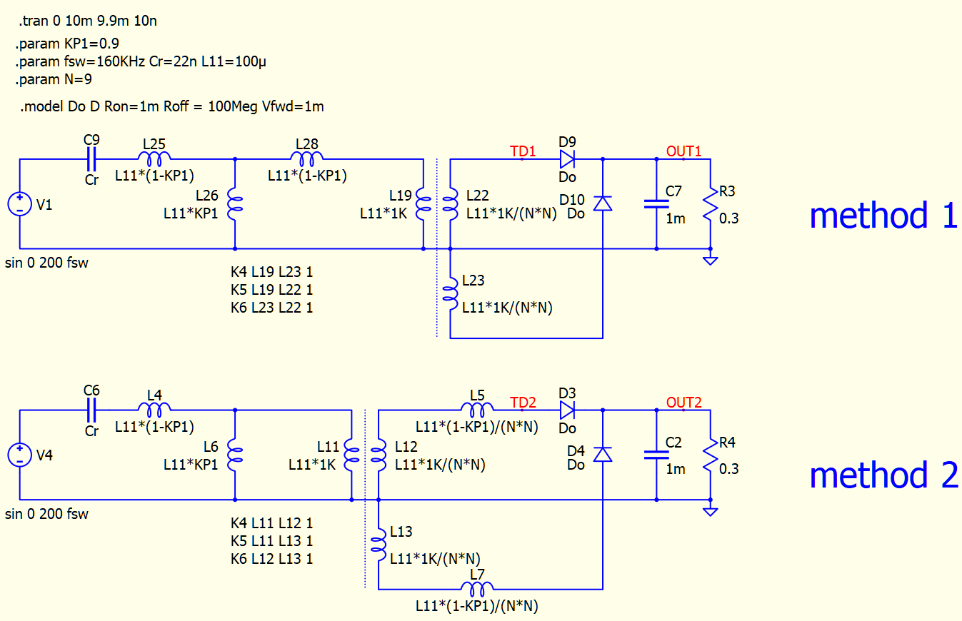
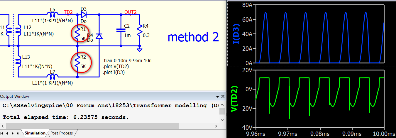
I am trying two different transformer modelling approach: T model but with secondary side leakage on the primary side or secondary side. The schematic is here: Transformer modelling_no image_.txt (17.4 KB). Picture of the circuit:
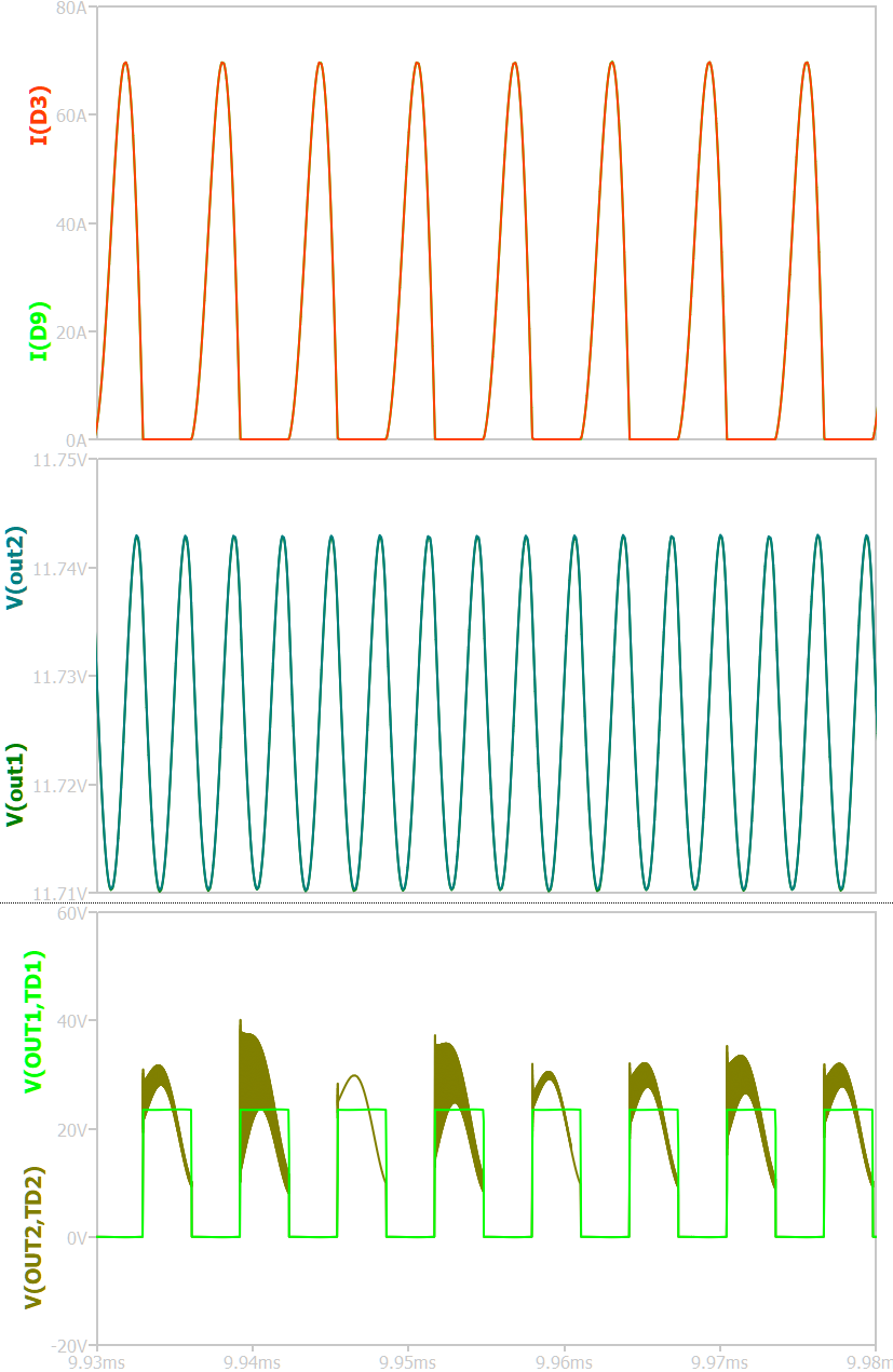
You can see that the output diode current and output voltage waveforms are almost identical of both methods (see below). However, the diode voltage waveforms are quite different. The method 2 where the part of leakage placed on the secondary side shows big oscillation. Here, the diode is pretty ideal. Questions are:
Why oscillaton happens on method 2?
Why the oscillation does not happen on each cycle?
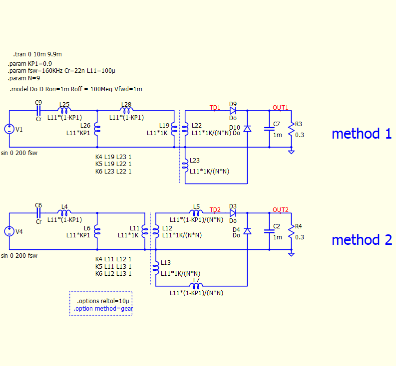
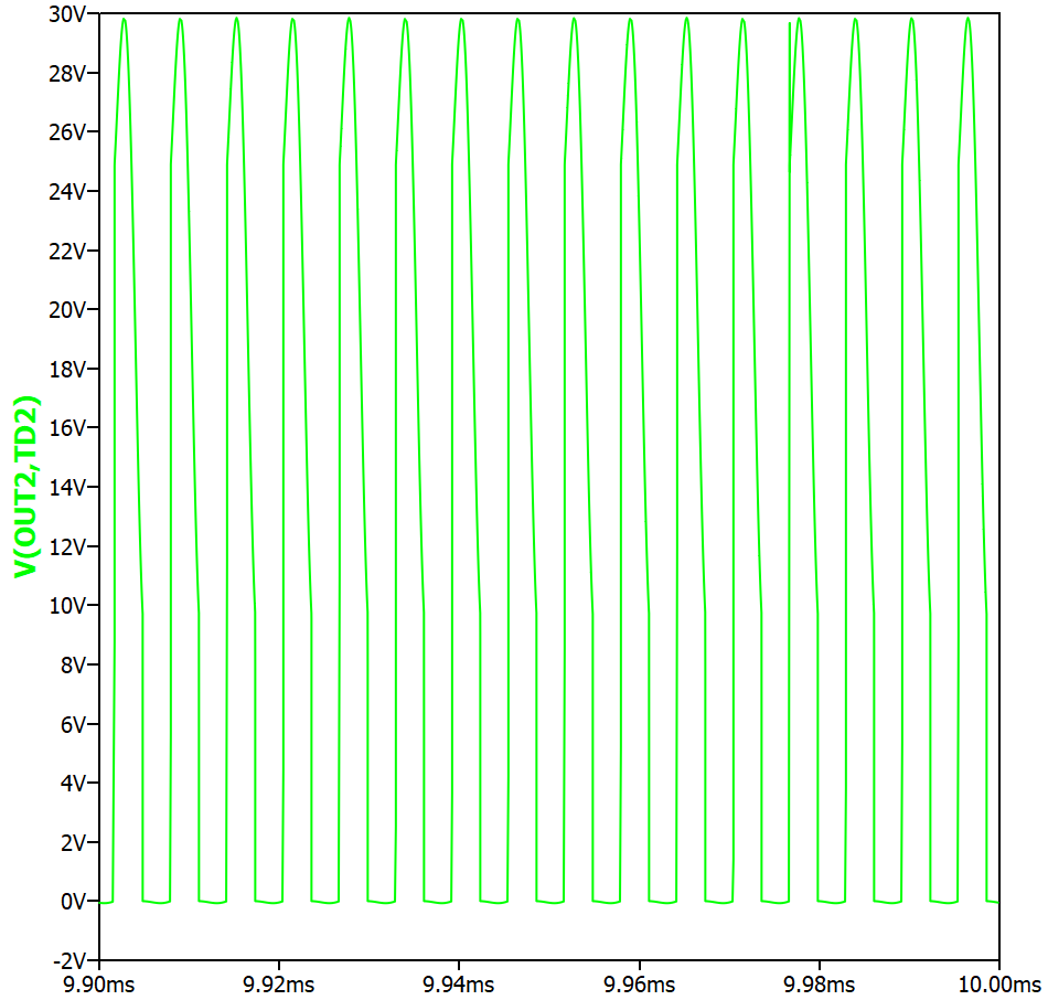
Hi Ivan, thanks for your reply. It reminds me this is a trapezoidal ringing. After looking into KSKelvin’s guideline material, I found it seems that trtol and trap method with feather can also help to remove the fake oscillation.
Then my question is: when to use what approach (reltol, trtol, gear method, trap method with feather) should be proper?
This is my understanding: Trapezoidal ringing may occur in simulations with ideal components, and its appearance suggests that practical circuits may experience ringing under practical conditions. I observed that this ringing commonly occurs when simulating circuits with an inductor and diode, particularly when the inductor current reaches zero (which is also when the ringing starts in your simulation).
As far as I know, there are three methods to deal with trapezoidal ringing:
Reduce timestep at breakpoints: This method involves reducing the timestep, nothing change in your circuit.
Add damping in the integration to dampen the numerical oscillation: This method requires adding damping elements to the circuit.
Post-processing data (Modified Trap): Mike proposed this method in LTspice, which is a post-processing approach (you can find more information in the LTspice help). However, Mike did not implement this method in Qspice, and based on discussions in this forum, it seems that Mike no longer wants people to be unaware of trapezoidal ringing.
By understanding these three methods, you should be able to differentiate between each approach:
Reduce trtol: This affects the timestep strategy and corresponds to method 1.
Trap with feather: This is a method used in HSpice to detune the trap integration and is possibly related to method 2.
Gear integration: This essentially changes the integration method, moving away from trapezoidal integration. Gear integration introduces artificial damping, but it is less accurate than trapezoidal integration. This is method 2.
Here is some additional information regarding dealing with trapezoidal ringing using your simulation example.
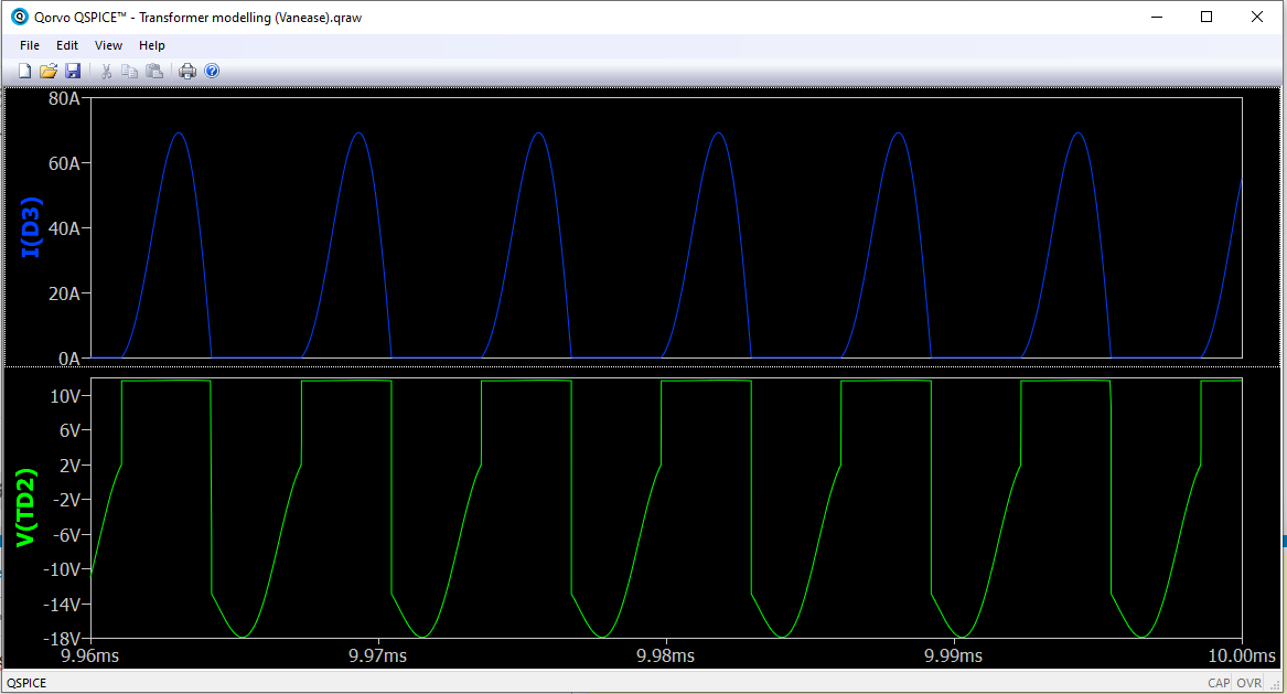
Based on your setup, it can be observed that trapezoidal ringing is closely related to instances when the inductor current reaches zero. Transformer modelling (Vanease).qsch (17.4 KB)
By adding a resistor, it is possible to dampen the numerical ringing by providing a “physical path” to dissipate the ringing Transformer modelling (Damping).qsch (18.7 KB)
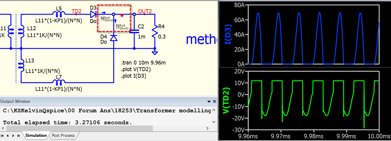
Here is a method I have considered: Since reducing the timestep can sometimes resolve trapezoidal ringing, it may be possible to achieve this by reducing the timestep specifically when the inductor current approaches zero. To implement this approach, I created a device that triggers the TTOL when the current approaches a reference value (in this case, 0A). This method can save simulation time by avoiding a reduction in the entire simulation step, while still helping to eliminate trapezoidal ringing. I have attached the symbol for your reference. (Please note that I have not documented this method, as I am unsure about its effectiveness in resolving trapezoidal ringing.) Transformer modelling (TTOL-device).qsch (19.0 KB) TTOL-I.qsym (671 Bytes)
Hi Kelvin,
Thanks for your comprehensive explanation! your TTOL-I device is interesting.
But about the simulation with TTOL device, your circuit gets the simulation done in 3.27 sec, but my computer makes it in 23 sec, 7 times slower. I know the different computer gives a different simulating speed, but on the “transformer modelling (vanease).qsch” my computer gives 8 sec, very close to yours in 6.23 sec.
Now I choose disabling the fast Math, it is one time faster but still 11 sec to finish. I will use another computer to try if any difference…let you know later
here: I just downloaded your file and simulate, in case I did any change on previous version.
I just install Qspice to my Dell Alienware m15 R2, and run that file with “Fast (less accurate) Math” disabled, and total elapsed time is 3 to 4 seconds. Similar to my working laptop Dell Latitude 5330. That interesting… as I expect this TTOL-device setup should run with less timestep as compare to force maxstep to 10ns. Let see what you find in your other computer.
I have tried two computers with Transformer modelling (TTOL-device).qsch and Transformer modelling (Vanease).qsch. HP-860G10, i7-1365U 2.69GHz, 32GB RAM:
…(TTOL-device).qsch: 16.5sec fast math enabled/ 8.3 sec disabled.
…(vanease).qsch: 6.3 sec enabled, 16.3 sec disabled.
In general, I see the simulation with the TTOL-device running slower. Additionally, with fast math enabled, the simulation with TTOL device runs slower but opposite in the …vanease.qsch case.
Dell Latitude 5330, i7-1265U, 1.8GHz, 16GB, Windows 10 Enterprise
…(TTOL-device).qsch: 8.1sec fast math enabled ; 3.3sec fast math disabled
…(vanease).qsch: 2.5sec fast math enabled ; 5.8sec fast math disabled
Dell Alienware m15 R2, i7-9750H, 2.6GHz, 16GB, Windows 11 Home
…(TTOL-device).qsch: 9.7sec fast math enabled ; 4sec fast math disabled
…(vanease).qsch: 3.7sec fast math enabled ; 7.4sec fast math disabled
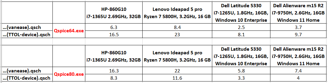
If I put all our test results for comparison, we can have this observation, which one is faster depends on which simulator is used.
Qspice64.exe (fast math enable) : …(vanease).qsch faster than …(TTOL-device).qsch
Qspice80.exe (fast math disable) : …(TTOL-device).qsch faster than …(vanease).qsch
You observation is correct, …(vanease).qsch with Qspice64.exe yield fastest simulation time in all computers, but this one with trap oscillation.
…(TTOL-device).qsch with Qspice80.exe is 2nd fastest in all computers, with trap oscillation eliminated.
we both run these simulation with same “relative” simulation time, our difference is “absolute” simulation time.
“fast math” is not guarantee “faster”, as here with a counter example that running …(TTOL-device).qsch can yield a faster result with Qspice80.exe (fast math disabled)
Yes, agree with your conclusions. “Fast math” does not guarantee a faster simulation. → What exactly does the “fast math” do with Qspice64.exe?
By the way, I have tried again on the Ideapad. When I plug in the power cable, then the simulation speed doubles. With the power cable in, … (ttol-device).qsch can finish in 5.1 sec with fast math disabled and 10 sec with fast math enabled.
Here is Mike’s explanation of Qspice64/Qspice80.exe. Qspice80.exe utilizes 80-bit math in critical sections. In the forum, you can find several cases where Qspice80 can produce accurate results while Qspice64 cannot, as these cases require higher-precision math. Personally, I changed my default to use Qspice80.exe. However, you can see from the post below that Mike recommends using Qspice64 as higher precision is rarely needed. Running qspice from command line? - QSPICE - Qorvo Tech Forum
It appears that your laptop limits its CPU clock in battery power mode. Great to know what slow down the simulation!
LTspice has similar problems with this circuit.
The best result I get is with a series RC network
connecting the anodes of D3 and D4. The values
of 100pF and 100 Ohm gave the best simulation
time: 2.461 seconds, alt. solver.
(Without the network: 16.82s.)
Your trick works quite well and I get the fastest speed from it so far.
Seems this realistic RC snubber gives the solver a chance to run away from the trapezoidal ringing with the ideal inductor and diode.
It happens because almost everything has been made lossless and ideal.
Speculation: When the simulator makes a small error in the on-time of the
output diodes, the secondary leakage inductor currents store some energy
that can go nowhere when the output diodes subsequently turn off again.
That is an error (more than) 2 timesteps back, and normal SPICE is only
able to reject the current timestep. The way to get the right results is thus
to make very small timesteps, which is correct but we don’t like the
consequences.
The RC circuit only works for superhigh-frequencies because of the small
value of the series capacitor and dissipates the excess energy in the
leakage without taking significant power from the load.
Trap-ringing is nothing special. Because the trap algorithm has an error
that oscillates between its min. and max. value instead of exponentially
decaying, the human eye “sees” this error. The trick of smoothing the
signal (modified-trap) is nothing but eye-candy (the error is still there).