Current imbalance with behavioural sources

[OHara]

I was trying to make a behavioural amplifier model that would respect power rails, following the advice to make device-currents continuous, and continuous in slope, with respect to node voltages, so as to avoid the “time-step too small” problems. The smoothed limiting functions I wrote did not help as I expected.

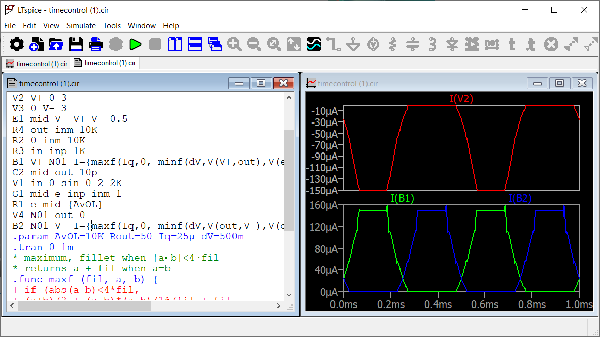
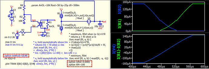
It looks like B-devices with .func-defined functions can put inconsistent currents in the output file, in that the total current into a node does not quite balance. The error decreases with shortened time-steps, so it might be something to do with which time-step is used for the inputs to the function.

timecontrol.qsch (12.6 KB)
I’m not quite sure how (or whether) to reduce it further to a minimal example for a bug-report, so I’m sharing here, to see if anyone has any insights.

[Edit : I suspect that the plotted I(B1) --with B1 being a current source-- is not accurate to the current source used in simulation, for the same reason that we cannot reference the current from a current source in other behavioural sources. There are comments on earlier posts about devices represented as ‘Norton equivalent’ (that is, parallel paths within the device, like a B current source) having the voltages across them solved by the Spice engine, but their currents then being ‘forensically’ figured out later by the plotter.]

[KSKelvin]

While probing I(V2) versus I(B1) current (expected to be identical), they showed different results, but the simulation has converged. I suspect that the unusual waveform in I(B1) is related to the V and I tolerances in the convergence criteria at each simulated timestep.

I conducted a test by tightening the tolerance by 10 times (.option reltol=0.0001), resulting in significantly improved results. I disabled the gear method as I prefer to observe trap ringing rather than using gear with damping during model development. I am uncertain whether I need to increase the maximum number of transient iterations since accuracy has improved due to reltol, where you may have higher opportunity run into convergence problem.

[KSKelvin]

I believe the reason adding maxstep can be helpful is because it reduces your simulation step size, and the “error” (I’m not certain if it can be referred to as an error) from the previous step will not be amplified too much in the next step.

However, the real reason for obtaining that unusual current profile is the allowable tolerance at each simulation step.

[OHara]

That is interesting.
RELTOL is only briefly described in Qspice and LTspice and Pspice docs.
NGspice says it will iterate to find a consistent set of voltages (the iteration done within a given timestep) until every branch current changes less than RELTOL of that current.
Spectre says it will iterate until the current balance at each node changes no more than RELTOL times the biggest branch current into that node.

When Newton iteration is near converging, the remaining error is well below the previous change. So I would think the default RELTOL=1m would iterate until these 100-µA currents are computed to 0.1µA, but the apparent discrepancy at the node was 20µA

I measured a couple currents with a 0-V V-device, and compared results with different RELTOL, those currents do seem to be converged within RELTOL. (When RELTOL is large the errors look more noisy than the imbalance plotted above.) It is only the reported currents through B-devices that are off more than RELTOL.

When I used .tran . . . <maxstep> to reduce the time-step, that would make each starting point for the Newton iteration closer to its eventual solution, so you might think each Newton iteration needed fewer cycles to converge. Maybe the closer starting point allowed Qspice to do better in figuring I(B1).

I still suspect something with I(B1) is being reported for plotting less accurately than the corresponding currents are computed. But, better to measure currents with 0-V voltage sources, which works in all flavours of Spice.

[OHara]

I figured out why smoothing I-V curves was not working as well as I expected.

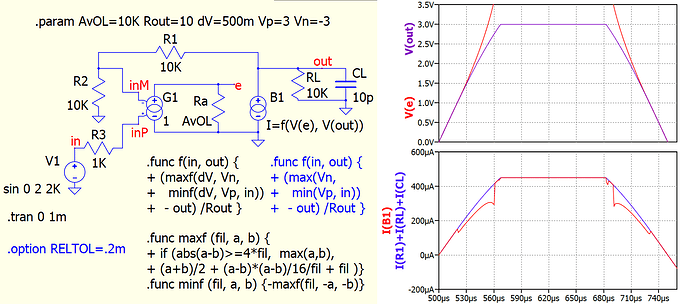
I decided to model the output impedance and voltage limits of a push-pull output stage as
I(B1) - I(B2) = (limit(V(e), V-, V+) - V(out)) /Rout
which has harsh corners when V(e) meets the power rails, with zero slope ∂I(B1)/ ∂V(e) outside the rails. That would not be good for Newton root-finding. I needed to add some load capacitance in the circuit above, or the simulation stops with small time-steps.

I thought smoothing the corners of the limit() a bit would let each Newton root-finding start somewhere with nonzero ∂I/∂V slope pointing the way to the solution, and thought rounding ±0.5 V around the corners would do the job.

But the Spice engine is not iterating to find the voltages at e and out independently; it is iterating a matrix solve, with each solve finding a set of voltages that balance all the currents in a linear approximation to the circuit.

The simple circuit above has an easy ‘matrix solve’ where in particular
V(e) = (V(in) - V(out)) AvOL /2
So the non-linear root finding is iterating to find a voltage at out to solve
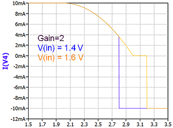
I(V4) = (limit( (V(in)-V(out)) × AvOL/2, V-, V+) - V(out))/Rout
where AvOL is typically 10k to 1Meg.

Rounding the corners of limit() did no good because the first argument to the rounded version of that function is a large voltage swinging very quickly through a narrow active area. I plotted the I-V curve as a function of guessed-voltage applied at out and it looks like the I-V curve of an op-amp using feedback to hold a voltage where it was told – no remnant of my smoothing is visible.

So I do need reasonable capacitance in enough places to limit how fast voltages swing in the model, so that the steep I-V curves I get in applications of the circuit don’t shift too much from one timestep to the next, giving Qspice a reasonable start at finding each solution.

[KSKelvin]

For the relationship between RELTOL, ABSTOL, and VNTOL, the most comprehensive explanation I’ve come across is in the “Behind the Scenes of the SPICE Circuit Simulator” lecture by Prof. Adam Teman. These three parameters are discussed in this Part 3 video at 4m15s.

Behind the Scenes of the SPICE Circuit Simulator - Part 3

I loaded your circuit into LTspice, and it gave the same result for I(B1) and I(B2), which suggests this at least not a unique characteristic in Qspice. Same as you, I also don’t quite understand why I(B1) and I(B2) seem to allow more tolerance than the rest. My guess is that SPICE solves the linearized matrix [G] [V] = [I], where the inputs are [G] and [I] to solve for the variable [V]. The B current source may be in [I] and not necessarily solved. I(V2) and I(V3) are different as they are voltage sources, and their currents will be added as variables into the [V] matrix for iteration, thus they are bound by convergence criteria. There is an example of modified nodal analysis explained by Prof. Adam Terman in his part 2 video at 13m8s. However, this is only my current speculation.

[OHara]

I might be too old for Youtube. I just get impatient and cranky.
I suspect they mis-spoke about the “sum of the residue current over all the nodes” Σ node_i being tested against tolerance, because that would ignore a current-error in a nonlinear element between two (non-ground) nodes. He is talking about Spectre, and their engineer’s explainer (p6) indicates that the current imbalance at each node is tested.

The best corresponding documentation that I found for Spice, so far, is the NGspice manual §1.4.2

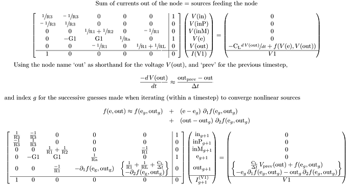
The Youtube video on nodal analysis is long and somehow still superficial, so I found the original paper on modified nodal analysis and applied it to the circuit above. That paper makes it clear, at the bottom of its second page, that tracking in detail the current from a current source is optional (surprisingly) and not recommended for the sake of speed.

So with the details as context, everything seems obvious:

• Qspice iterates until each voltage is stable to ±0.1%
  so at some timestep the iteration might tell us V(e)=3.000V±3mV
  and at the same timestep it happens to tell us that V(out)=2.496V±2mV
• Qspice figures my well-intentioned soft minimum minf(dV, 3V, e)=2.500V
  and the difference between that result and V(out)=2.496V±2mV, which is 4mV ±2mV
• The calculated current through B1 has a large relative uncertainly, because it is the difference between the two voltages that Qspice tested for tolerance.

Both Spice and Spectre check that all the voltages, and I(V1), in that column vector have converged.

As I understand the Spectre criteria for convergence, they would also put the final voltages, ‘out_(g+1)’ etc., into the nonlinear function f(e_(g+1),out_(g+1)) and re-check the matrix equation. (The terms with the partial derivatives ∂ all cancel if we have g+1 on both sides) Now, the matrix solve found voltages that exactly solve the matrix equation for the linear approximation to f(e_(g+1),out_(g+1)), based on evaluations at e_g, etc., so this is a way to see how well that linear prediction held true. It seems this test would have checked that my B1 also came out within specified tolerances.

The NGSpice docs say they also check convergence of currents through nonlinear devices, but for each branch going into a node, which seems they are being more careful if there are many branches with nonlinear elements feeding one node. Reading carefully, NGSpice don’t say they figure the nonlinear function at the final voltages, f(e_(g+1),out_(g+1)), but only that the final update, g to g+1, made a small change, given the linear approximation using derivatives at iteration g. I do not want to need to worry about such details.

Moral: use zero-volt voltage sources to have Spice report currents, like the Spice textbooks tell you.

[Edit: The issue with I(B1) being more inaccurate than RELTOL implies, does seem to violate the promise of SPICE as described in the NGspice user manual. Also, the NGspice source code (which is close to the original core SPICE) seems to have an error in its convergence check, affecting only B-devices, not real devices, so I’ve submitted a bug report there (with a very simple circuit deviously designed to be difficult for Newton’s method, to help isolate the issue). ]

[bordodynov]

OHara,
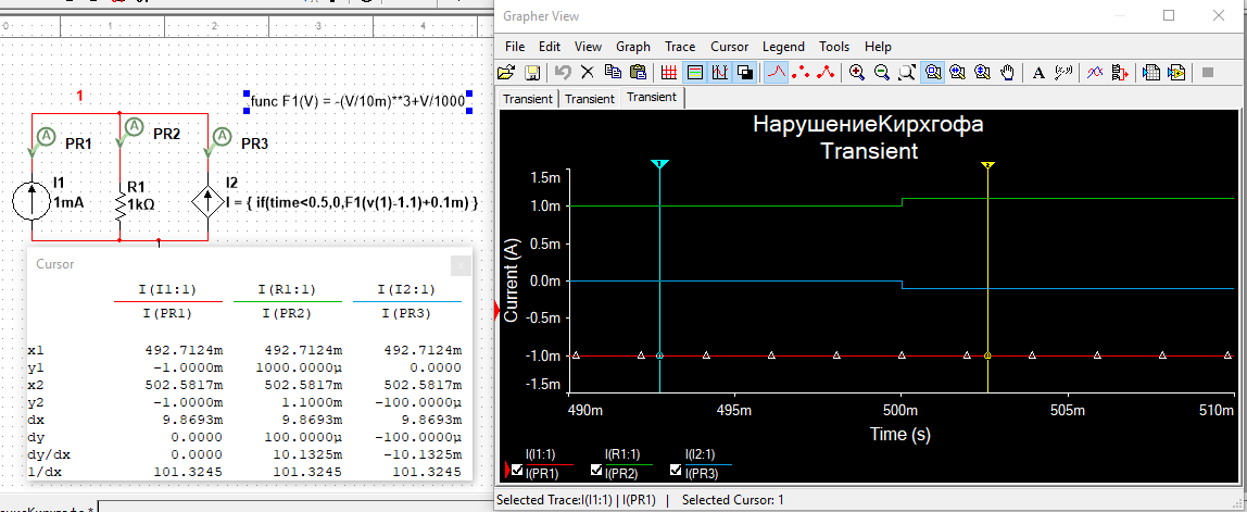
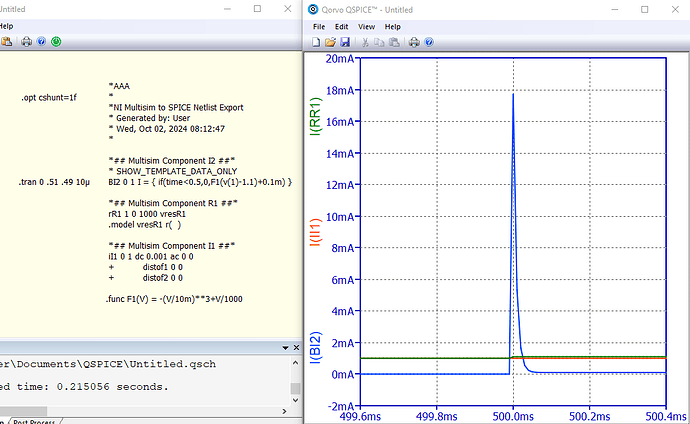
I decided to see how Multisim will manifest on your electrical circuit. I criticize this program all the time. What was my surprise that Multisim proved itself worthy in this case. To correctly enter the scheme into the Multisim, I extracted a list from its scheme and modeled it in Qspice.

[OHara]

@bordodynov

Multisim proved itself worthy

That is interesting. It looks like Multisim is converging within each timestep as it should (which only takes a few extra Newton root-finding iterations, if the simulator notices the iterations are needed). And, the Multisim documentation also says its default RELTOL=1m.

I see the same logic (that I suspect to be in error) in the code of Spice3f5 from berkeley.edu, but I haven’t set up to compile spice and test, so maybe I have the wrong cause. If NI fixed the error, they should have provided the fix upstream.

Anyway, almost always, the convergence tests on node voltages and all the other devices (like zero-volt sources for current probes) will keep iteration going until true convergence.