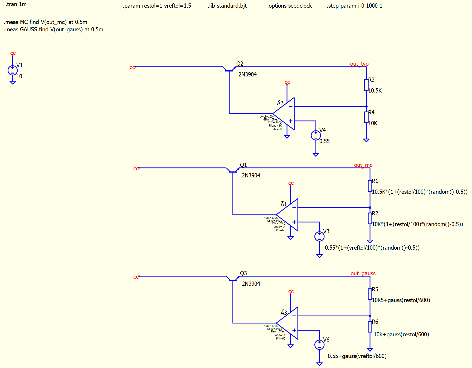
as I was struggling with this a bit in the beginning, sharing this might help someone. Goal was to model a output voltage spread of an LDO varying the Vref=0.55V (1.5% tolerance) and divider resistors (1% tolerance).
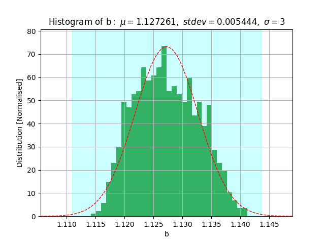
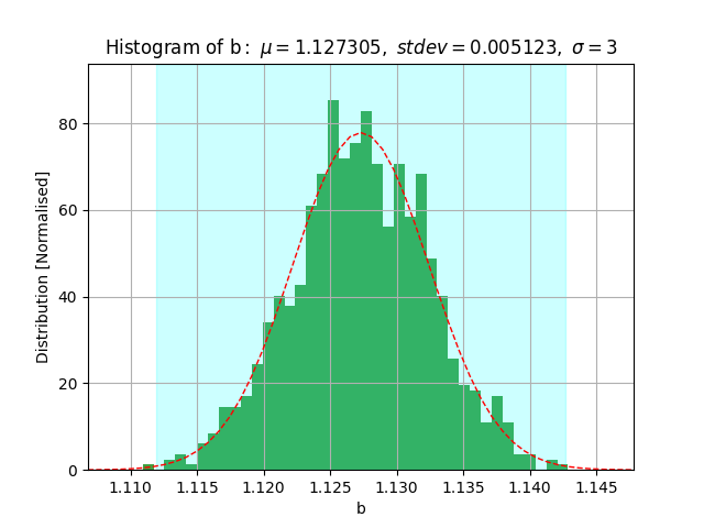
I was interested how the results differ when using “random()” function or “gauss()” function. In the case of gauss() the argument is sigma and the percentage of tolerance is considered as 6sigma. Therefore the argument is (tol/600).
The typical Vout value (no component variation) is Vout=1.275V
I also used Python scipt (credit: PyLTSpice · PyPI) to create the histograms.The visual difference between the results is apparent
Hereby I’d like to suggest to Mike @Engelhardt making the .meas output more machine-processing friendly. I needed to do some manual editing after every simulation to be able to process with python script. Option of some basic .csv- type output would be greatly appreciated.
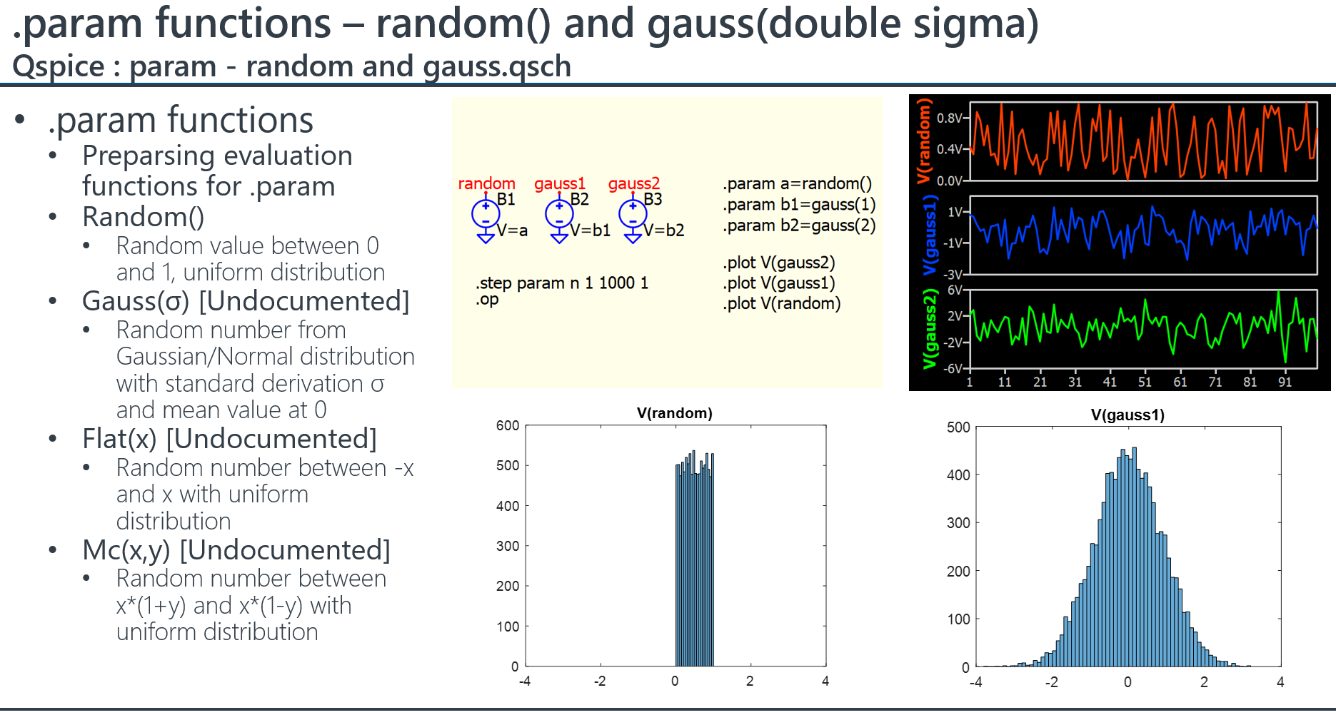
From your implementation, it appears that you may not be aware that Mike has implemented functions that could simplify your formula. Some of these functions may be undocumented, but you can find their implementation in the revision history.
Random() : Random value between 0 and 1, uniform distribution
Gauss(σ) : Random number from Gaussian distribution with standard derivation σ and mean value at 0
Flat(x) : Random number between -x and x with uniform distribution
Mc(x,y) : Random number between x*(1+y) and x*(1-y) with uniform distribution
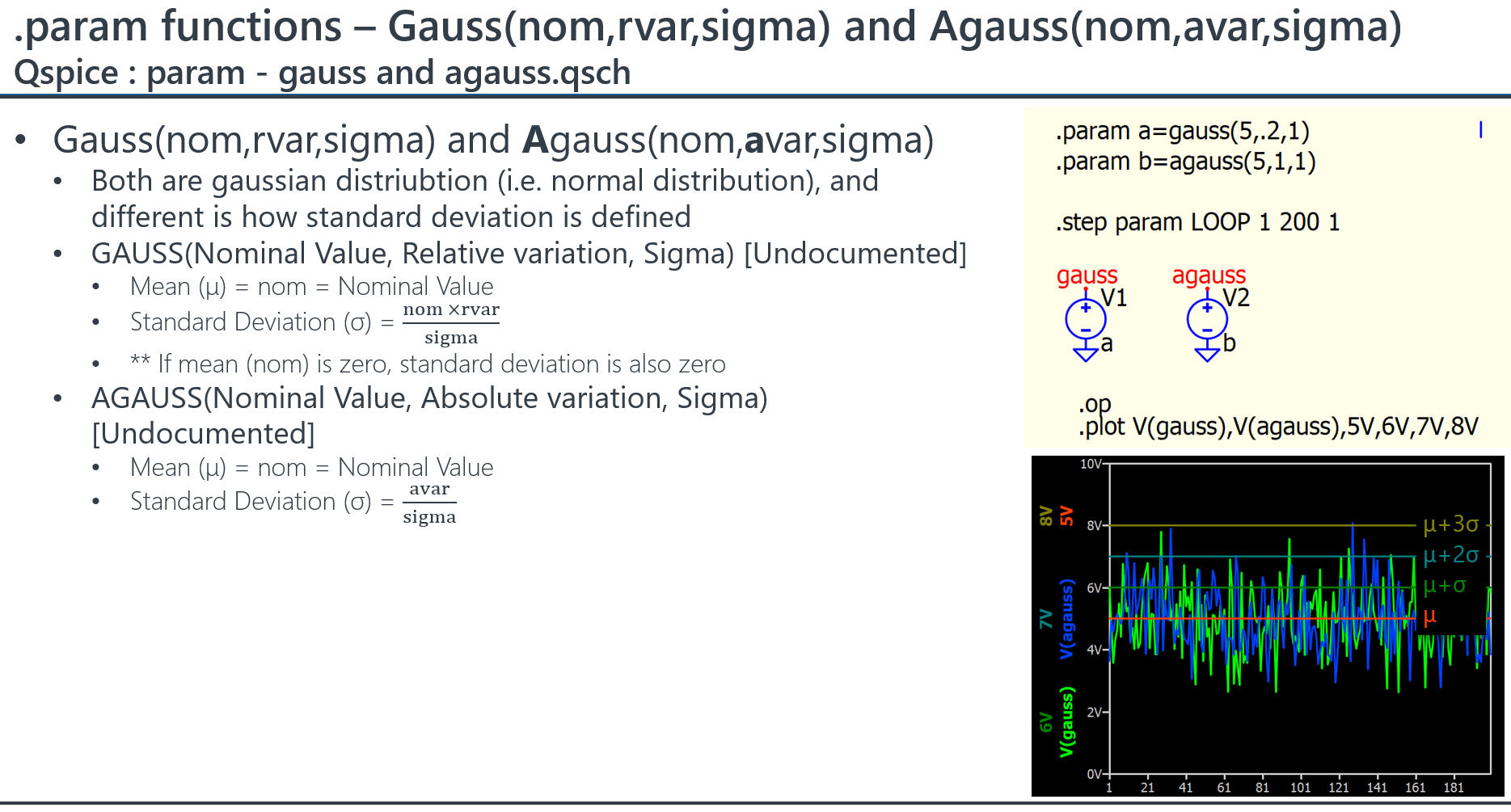
GAUSS(Nominal Value, Relative variation, Sigma) [refer to below example]
AGAUSS(Nominal Value, Absolute variation, Sigma) [refer to below example]
Hello, trying to follow along, since I have a simulation for which I want to run a montecarlo analysis of sorts. When you say “in the case of gauss() the argument is sigma and the percentage of tolerance is considered as 6sigma” is this your definition, or how the gauss() function defines the percentage of tolerance? I’m struggling to find any documentation on the usage of these functions…
Gauss and Agauss description can be found in Qspice Revision History 05/08/2024 Implemented GAUSS(Nominal Value, Relative variation, Sigma) and AGAUSS(Nominal Value, Absolute variation, Sigma)
Gauss accepts two type of format, Gauss(sigma) OR GAUSS(Nominal Value, Relative variation, Sigma).
In my documentation, I input values into formulas to verify their meanings. Here is a schematic you can use to test the functions yourselves. Just be cautious that in GAUSS(Nominal Value, Relative variation, Sigma) and AGAUSS(Nominal Value, Absolute variation, Sigma), the third argument known as Sigma is NOT the standard deviation. I believe the slide in my previous post highlighted the formula.
Or, you can utilize AGAUSS() and consistently set the second argument (absolute variation) to 1, where the nominal value represents the mean and sigma represents the standard deviation.
In statistics, 6sigma equates to 6 x standard deviation. Therefore, approximately 99.7% of the data falls within ±3 times the standard deviation. It seems there might be confusion regarding the term ‘sigma = standard deviation.’ in Qspice AGAUSS() and GAUSS() formulas, as Sigma (the third input argument) does not directly represent the standard deviation.
(remark : but GAUSS(sigma) where only one argument format, this sigma is a direct standard deviation)
GAUSS() and AGAUSS() definitions can be found in the HSPICE user guide. You can locate the explanation of these functions in Appendix A > .PARAM Distribution Function
thank you.
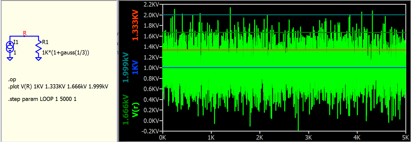
So, if I use R1 = 1k*(1+gauss(1/3)), what would the maximum possible value of R1 be? As I understand it, gauss(1/3) is making making 1 standard deviation = 1/3 or sigma= 0.33. So, 6 std dev would be 1.98…does this mean that 99.99966% of the time, the value of R1 will be less than 2.98k?
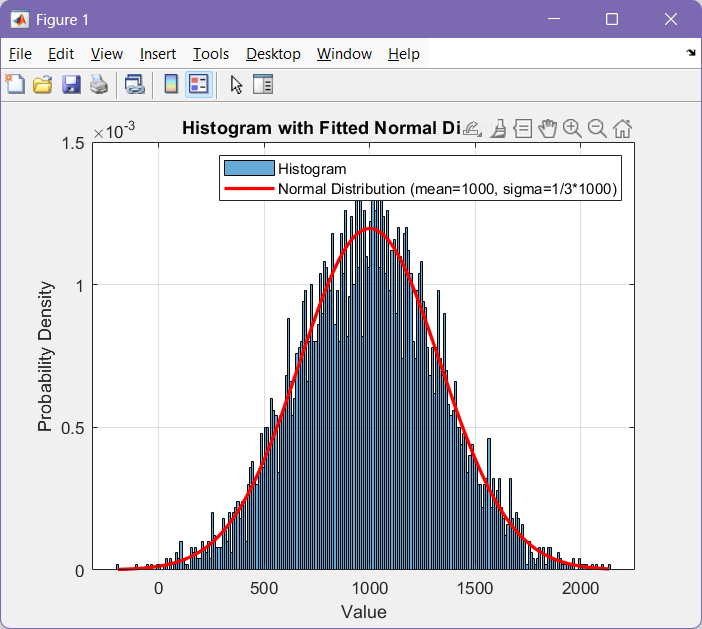
There is no maximum/minimum possible value in a gauss distribution, just the probability extreme low. Here is an example to run your equation 5000 times and compare to normal distribution curve with mean=1000 and sigma=1/3*1000.
To ensure resistance not becomes negative or excess 2kohms, use this formula to force a lower and upper limit. Any gauss generated results < 1m is limited to 1m, and >2k is limited to 2k. limit(1K*(1+gauss(1/3)),1m,2K)