How can I simulate the gaussian distribution

Hi ,

How can I simulate the gaussian distribution (normal distribution in Qspice). I came accross this post while searching the method
Simulating tran noise with QSPICE - QSPICE - Qorvo Tech Forum

I have plotted the histogram of the method in the post. However, it does not look like the normal distribution to me.


PyQSPICE


Here is how you simulate gaussuan distribution.


Best regards

Hi Ivan,

Thank you for the solution. Is there any way I can do it in the transient analysis? I want to see how my circuit react to noise.

Regards,
Joe

This is a workaround, by adding 6 random calls to make gaussian look alike distribution.

V=random(time)-random(time+17)+random(time+27)-random(time+37)+random(time+47)-random(time+57)


This is the best I can think of in generating a gaussian distribution in .tran and can follow gaussian distribution in regardless simulation time.

SrcGaussian.qsym (2.2 KB)
example.SrcGaussian.qsch (3.2 KB)

** if you enable .option seedclock, it can generate new set of random number in each simulation run.

Here is netlist of this .subckt for your reference

.subckt X1•SrcGaussian Y0+ Y0- Y1+ Y1-
B1 U1 0 V=limit(random(1e15*time/V(divider)+1e15*random()),1m,0.999)
B2 U2 0 V=limit(random(1e15*time/V(divider)+1e15*random()),1m,0.999)
B3 Z0 0 V=sqrt(-2.0*log(V(U1)))*cos(2.0*3.14159*V(U2))
B4 Z1 0 V=sqrt(-2.0*log(V(U1)))*sin(2.0*3.14159*V(U2))
B5 Y0+ Y0- V=mean + std * V(Z0)
B6 Y1+ Y1- V=mean + std * V(Z1)
B7 divider 0 V=pow(10,floor(log10(time)))
.ends SrcGaussian
1 Like

Thanks Kelvin…You’re the best…

@physicboy I saw your question in previous post. Here is more information for your reference.

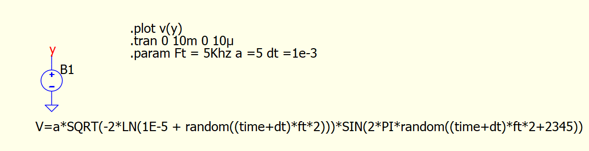
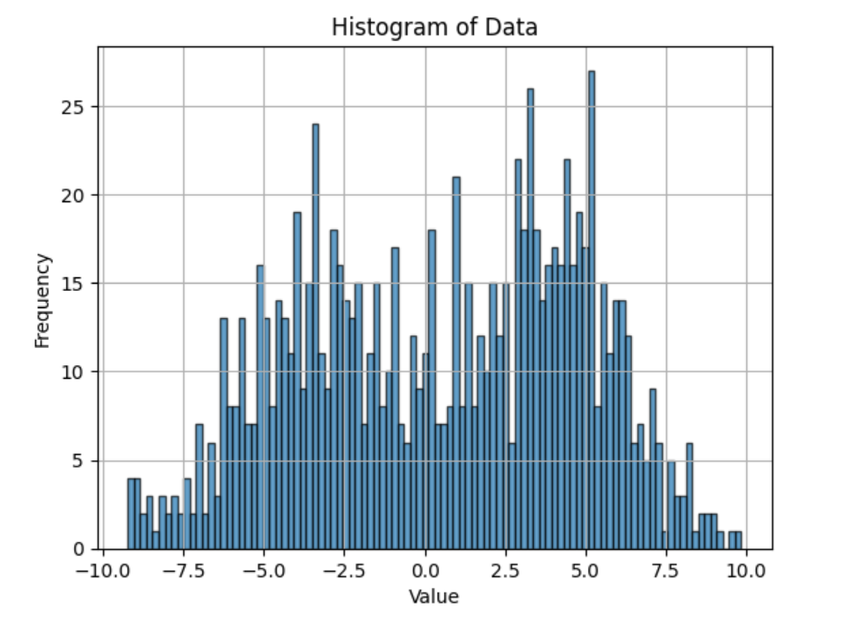
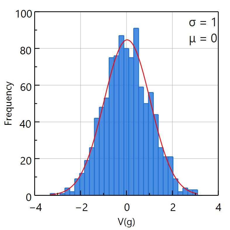
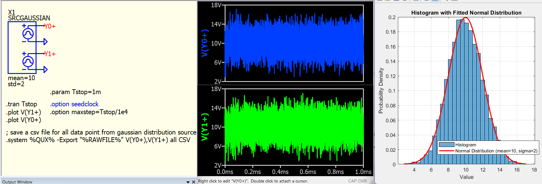
This method is called Box-Muller Transform (Box–Muller transform - Wikipedia), it based on two set of uniform distribution random number to generate two set of gaussian distribution data.

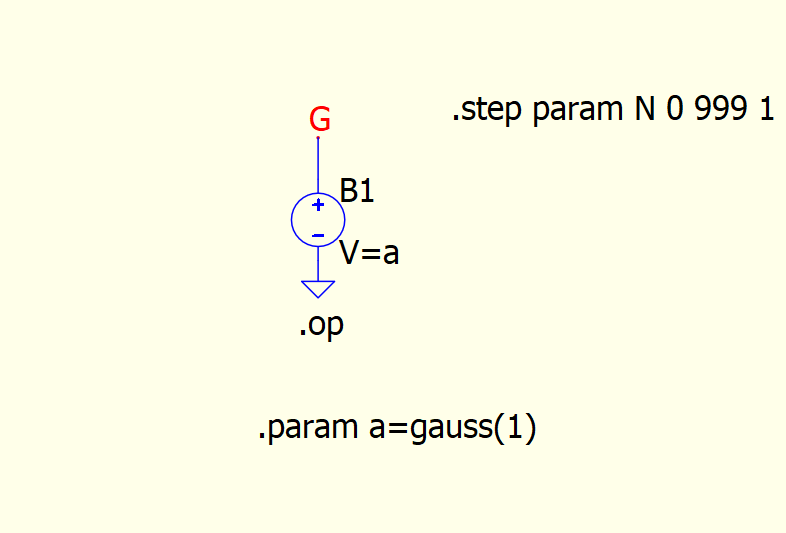
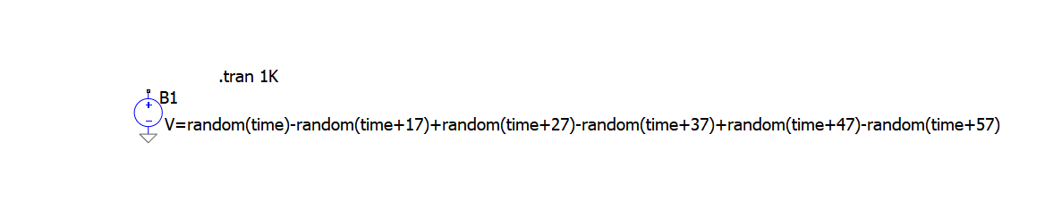
Additionally, for the uniform distribution random generation, the formulas in B1 and B2 appear more complex because to truly generate a random number with a uniform distribution, the seed within the random() function needs to be between 0 and 1e15 (or 1e16?). During simulation, we typically use the simulation time as a pseudo seed. However, time alone does not fall randomly within the range of 0 to 1e15, so we have to multiply it. Nevertheless, a challenge arises because time can vary for example from 1us to 1s. Therefore, even if I multiply by 1e15, the result can still be significantly lower than 1e15 if for example in 1us range. This discrepancy leads to a non-uniform distribution of random numbers. Therefore, @mingche_joe cannot see a distribution looks like gaussian distribution. This is why a divider is employed to ensure that time always cycles within the range of 0 to 10, and the time seed can always within 0 to 1e15 to help random() function to generate a uniform distributed data.

The 1e15*random() in the seed is to help generate an offset in seed, and this offset can change everytime if .option seedclock is enable.

I hope this clarifies what I am doing here

Thanks Kelvin for the detail explanation

By the way, a bit different question

Is B-source random just give us Pseudo Random Binary sequence with some low pass filter?