Erroneous results from D(V(out)), & .meas D(V(out))

[Avinash]

Hi,
Kindly refer to the attached simulation file ‘ExportedData.qsch’ which simulates a PWL file [ Data.csv ]. I 've found some very disturbing results from the same which I discuss below:
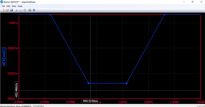
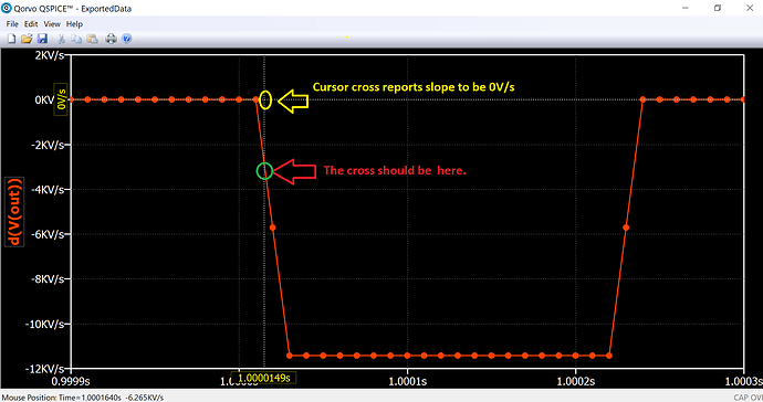
A) Take a look at Dout.bmp which shows how cursor cross is NOT a faithful representation of the plotted data. One can see cursor cross way below the flat portion of d(V(out)). It is not in alignment with the plot. In fact, if one drags it along the flat portion of D(V(out)), the coordinate is reportedly varying while one can see that it should be a constant value.

B) If one takes help of mouse position, then d(V(out)) in flat portion is around -407. This value is different from what the cursor cross reports as one can see from point A above. Moreover, this -407 itself is wrong value. To see that, see out.bmp which shows V(out) as well. To calculate the slope, i am relying on mouse position [ as cursor reports a wrong value as discussed in point A]. I get slope as -2.4/(1.0023 - 0.999358) = -815.771584.
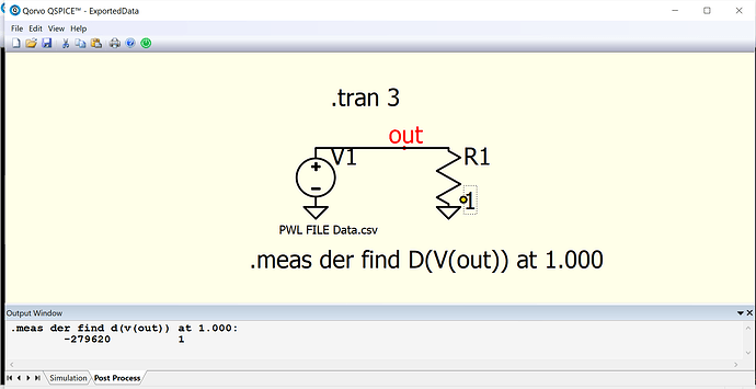
C) Finally, the .meas der find d(v(out)) at 1.000 yields -279620 !!!.
So, the value reported by .meas is also wrong, and is different from the plotted d(V(out)) which in turn is also wrong, as well as different from what the cursor cross shows.

Clearly, this begs attention of concerned people. Kindly let me know, if the undersigned is missing something obvious here.

Neverthelss, Thank You so much for your patience to hear me out.

Thanking You
Data.csv (217.9 KB)

Data.csv (217.9 KB)

ExportedData.qsch (1.5 KB)

[OHara]

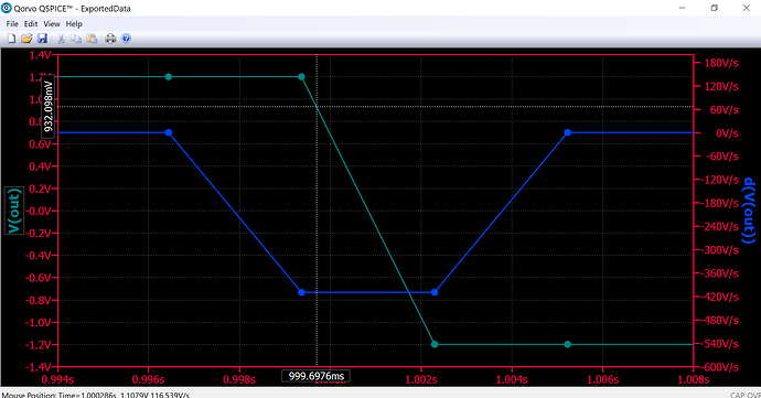
I understand why you are surprised. Qspice resamples the data from your file.

In general it will be simulating some complex circuit (given the piece-wise linear input specified in your file) and deciding as it goes how densely in time to sample, based on how fast the circuit is changing.

Your input file has breakpoints spaced by about 200µs, given time(s) input(V) :

0.99981,1.2
1.00002,1.2
1.00023,-1.2
1.00044,-1.2

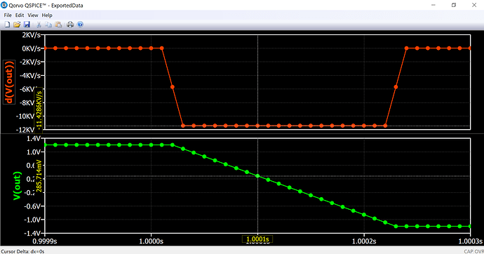
so D(V(input)) is clearly 0V/s at 1s, but −11 kV/s between 1.000 020 s and 1.000 230 s.

In the QSpice plot we see in the plot about one sample every 2 ms, so the plot misses the sharpness of the transition. It looks as if QSpice got bored waiting for something to change in that simple circuit.

The cursor behaves in a reasonable way (to me) for purposes of examining samples of voltages and currents along a smooth curve. If you hold the cursor at the middle of the step between samples, the D(V(out)) cursor does show the value you calculated. The nearest plotted points are halfway on the slope, halfway on the flat, and show just half the slope.

The documentation suggests PWL FILE Data.csv TIMECTRL=BREAKS if you want at least one simulation point for every breakpoint in the input file, but QSpice still speeds up over all those repeated equal values in the input.

You can ask the simulator to take smaller steps .tran 0 1.025 0.975 20u and see the plot you probably expected.

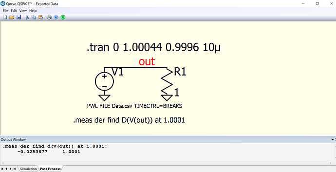
The .meas result is still incorrect, though.

[Avinash]

@OHara , Thank You so much for your suggestions, and detailed analysis of the issue.
1.The suggested changes does address the issue of wrong value of slope.

2. But the issues mentioned in point A, C [ original post ] remains. The correct slope of -11428.57143 V/sec [ based on data.csv ] at t=1.0001sec is not reported by .meas. Secondly, the mismatch between cursor-cross and actual value seems to be in direct proportion to how coarse the simulation is. One can observe this issue in the figure shown below, and also in Dout.bmp of original post.
   
   

Anyway, thanks again for everything.

[KSKelvin]

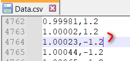
In Data.csv, the derivative you would like to measure is at this location

Derivative can be calculated with finite difference derivation, in backward direction
i.e. = (-1.2-1.2) / (1.00023-1.00002) = -11428.6 @ t=1.00023s

I have a symbol that implement the backward finite difference derivative, which can yield this measurement result. SPICE cannot look into future, and we cannot calculate forward finite derivative during simulation, therefore, at t=1s, if you look backward, derivative is still zero. Therefore, the measurement has to be taken at 1.00023s

As @OHara reminded, you also need to force simulation point for every breakpoint in the input file by including TIMECTRL=BREAKS

Here is the simulation file and this math symbol for your reference

Data-FiniteDerivative.qsch (3.1 KB)
FiniteDifferenceDerivative.qsym at KSKelvin-Github

Actually, Qspice stanard ddt() function in B-source actually yield this same result. Therefore, I guess ddt() basically backward finite difference derivative.
You just have to be careful that thinking at 1s can give the derivative you want is NOT correct in backward derivative.

I am not sure what the math is for d() in post-processing does, at least it is not backward finite difference derivative. But not knowing that doesn’t mean it is incorrect, as d() is in post-processing and it can take future data into account.

[OHara]

I agree, @Avinash, that the plot for D(V(out)) looks strange.
I was merely less surprised or disturbed, because I recognize the strange thing it is doing. Calculating derivatives is tricky, and the correct method depends on what needs to be done with the output, so there is a small chance Qorvo might need to keep D() this way.

It appears that D(V(t)) is doing a centred difference, when t is centred between samples, and interpolating linearly between centred differences for other times t. I don’t find the formula very helpful, but if t_n is the nearest sampled time
[ (t_n + t_n+1 − 2 t) × (V_n − V_n-1) / (t_n − t_n-1)
−(t_n-1 + t_n − 2 t) × (V_n+1 − V_n) / (t_n+1 − t_n)
] / (t_n+1 − t_n-1)

The cursor on D(V(t)) does this differencing for any t, so when you put it at the centre of a flat portion it shows 0 V/s (which is correct from looking at the V(t)). The plot, however, has dots at the sampled times, not the centred times, and draws lines between those dots.

We all agree that the .meas <n> find D(V(t)) output is way wrong. The meas <n> deriv is also wrong:

.meas der find d(v(out)) at mtime:
     0.00017035     1.0001
.meas deriv deriv v(out) at mtime:
     0.00017035     1.0001
.meas ddt_circuit find v(ddt) at mtime:
       -11428.6     1.0001
.meas c_curr find i(c1) at mtime:
       -11428.6     1.0001

There were many many extra lines in the data.csv, and I wondered if they were confusing Qspice, so I removed the extra lines, but see no difference in the behaviour we are talking about.
Data_trim.csv (327 Bytes)

[[ Edit: I emailed a formal bug-report about meas deriv to the address on Qspice::Help.

* Expected 'meas der' below to report -2π·1000 V/s
* `.meas <n> deriv <x>` anywhere in the deck seems to corrupt <x>
V1 q 0 sin 0 1 1K
C1 q 0 1µ
.tran 1m
.meas V find V(q) at 0.5m
.meas der deriv V(q) at 0.5m
.meas C_curr find I(C1)/1µF at 0.5m
.end
===
.meas v find v(q) at 0.5m:
        11766.8     0.0005
.meas der deriv v(q) at 0.5m:
        11766.8     0.0005
.meas c_curr find i(c1)/1µf at 0.5m:
       -6283.19     0.0005

context at Erroneous results from D(V(out)), & .meas D(V(out)) ]]

[Avinash]

Very many thanks to @KSKelvin, and @OHara for offering their time and attention to this problem. Let me gather what I understood from all this:

A) Cursor-cross not in alignment with plotted points in some interval of time:
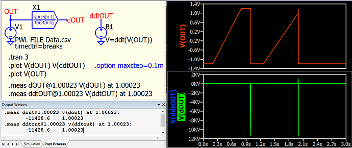
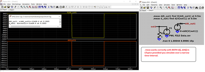
I think, @OHara has nailed this issue: the algorithm used by plot, and cursor seems to be different which is why they are at variance over a time-interval. Both @KSKelvin , @KSKelvin kindly suggested the possible algorithm that these utilities might be using. I found the same issue with LTspice also. Here is the snapshot:

B) Wrong value of slope reported by cursor, and or plot:
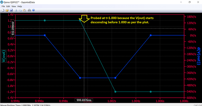
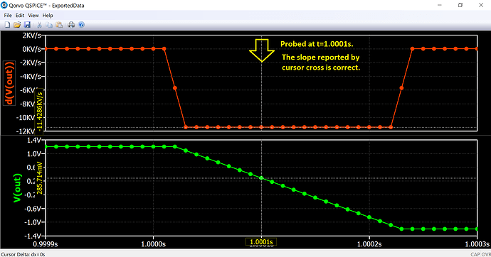
Again, @OHara sealed this issue by suggesting to do .tran over a narrower range of time. Agreed. Followed his suggestions in my previous post, and got correct results. I probed at t=1.000s in first post because :

In the 2nd post, I probed at t=1.0001s because:

It is NOT correct, IMHO, to suggest probing at t=1.00023s because, you should be getting the same slope at t=1.0001s itself as per the plot. The user looks at plot, and not the underlying data. This data is itself generated by QSPICE from some other simulation file.

However, that being said, the utility shared by @KSKelvin is really useful because there is no documentation about encapsulating a algo/circuit/dll into a sub-circuit. I will have to learn from his older posts about the procedure to make such utilities.

C) .meas gives wrong results with d():
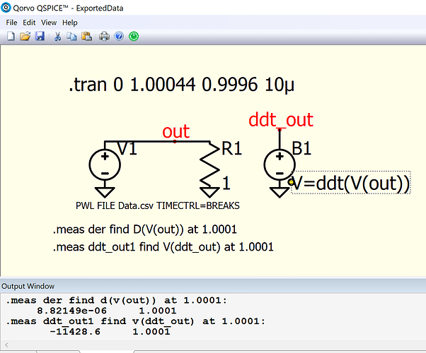
@OHara, and @KSKelvin both suggested using ddt. Here, I would like to share the following two figures, one with LTspice, and other with QSPICE. The figure conveys the message I wanted to conclude:

So: d() of QSPICE returns wrong results with .meas whereas .meas with ddt gives right result: it means they are following different algorithm. d() is used in post-processing, and so, it can always look into future, history, and wherever it wants to. I don’t know why it gives wrong results. This conclusion resonates with findings of @OHara.

Let’s check how LTspice fares on this issue. Here goes the finding:

Wow!!, both d(), ddt() gives same, and correct result with .meas in LTspice.
PS: I probed at 0.5ms in LTspice file because t=1.0001 is 0.5ms away from tstart=0.996s which is where I stared the .tran simulation in LTspice following suggestions of @OHara. LTspice labels tstart to be 0sec.

So, I thank all concerned for offering their precious time to this seemingly simple but pertinent issue. I would use ddt() rather than d() if working in QSPICE.

Thanks again.

[KSKelvin]

To create embedded sub-circuit symbol from hierarchy, I have a tutorial in my General Reference Guide, which can download from this GitHub link. Goto section Part 2B, subtitle “Procedure to Create embedded SUBCKT symbol from Hierarchy : Method #1” (currently page. 33 to 34)
Qspice/Guideline at main · KSKelvin-Github/Qspice · GitHub

This is a latest demo from Mike, talking about creating a symbol from sub-circuit netlist, from 1h0m35s

Webinar QSPICE latest simulation tool by Mike Engelhardt.