DIY UWB Precise Positioning with Downlink TDOA

BD8NCF · May 15, 2026, 3:51pm

1. Introduction

Previously, I wrote several articles about building a UWB precise positioning system using TDOA technology from scratch. The TDOA technique described in those articles was Uplink TDOA. Recently, I completed a full implementation of a UWB precise positioning system based on Downlink TDOA technology. During my research on Downlink TDOA, I published several related articles. Now, I am consolidating all the information and combining it with recent insights into this comprehensive article.

This article is written for hardware and software engineers who have embedded development experience but no prior UWB positioning background. Therefore, before diving into system design, I will spend some time covering the fundamentals of UWB and TDOA positioning. If you are already familiar with these topics, feel free to skip ahead to the sections that interest you.

1.1 UWB Overview

Before getting into the TDOA positioning principle, let’s first introduce the basic concepts of UWB (Ultra-Wide Band) to help engineers without a UWB background quickly build a foundational understanding.

What is UWB?

UWB is a short-range wireless communication and ranging technology. It is governed by the IEEE 802.15.4z standard (published in 2020, which enhanced security and ranging accuracy based on the earlier IEEE 802.15.4a standard). UWB is fundamentally different from traditional WiFi and Bluetooth:

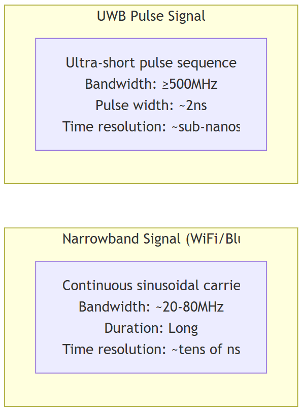
WiFi/Bluetooth use continuous sinusoidal carrier waves to transmit data, with the receiver demodulating the carrier to recover information. These signals typically have bandwidths of only a few tens of MHz (an 80MHz WiFi 5 channel is already considered wide).
UWB uses extremely short pulses (typically sub-nanosecond to a few nanoseconds wide), with signal bandwidths of 500MHz or more. It’s called “Ultra-Wide Band” precisely because of this enormous bandwidth.

Here is a simplified comparison between these two types of signals:

Why does “wider bandwidth” mean “better positioning accuracy”?

This can be understood from both time-domain and frequency-domain perspectives:

Time-domain perspective: The narrower the pulse, the higher the resolution on the time axis. UWB pulse signals can resolve down to the sub-nanosecond level. Since electromagnetic waves travel at the speed of light — 1 nanosecond corresponds to approximately 30 centimeters in air — if we can precisely measure signal arrival time, we can theoretically achieve centimeter-level distance measurement.

Frequency-domain perspective: According to signal processing theory, the wider the signal bandwidth, the higher its time-domain resolution (i.e., the ability to distinguish two closely spaced signals). A 500MHz bandwidth corresponds to a time resolution of approximately 2ns, or about 60cm of spatial resolution. The chip’s internal oversampling and interpolation algorithms further improve actual precision well beyond this theoretical limit.

In comparison, WiFi signals have bandwidths of only a few tens of MHz, corresponding to several meters of resolution — this is why WiFi-based positioning (using RSSI or RTT) typically achieves only 1–3 meter accuracy, while UWB can easily achieve 10–30 centimeters.

How UWB Works — The Thunder Analogy

If you’re not yet clear on “time-based positioning,” imagine a thunderstorm: Lightning occurs instantaneously (light-speed propagation means virtually no delay), and only afterward do we hear the thunder (sound travels at approximately 340 m/s). By measuring the time difference between seeing the lightning and hearing the thunder, we can estimate how far away the lightning struck. UWB positioning works on a very similar principle, except we’re capturing electromagnetic pulses rather than sound waves. Since light travels extremely fast (approximately 3 * 10^8 m/s), the UWB chip’s internal timer must have extremely high resolution to precisely capture these brief time-of-flight differences.

The DW3000 Chip’s Timer

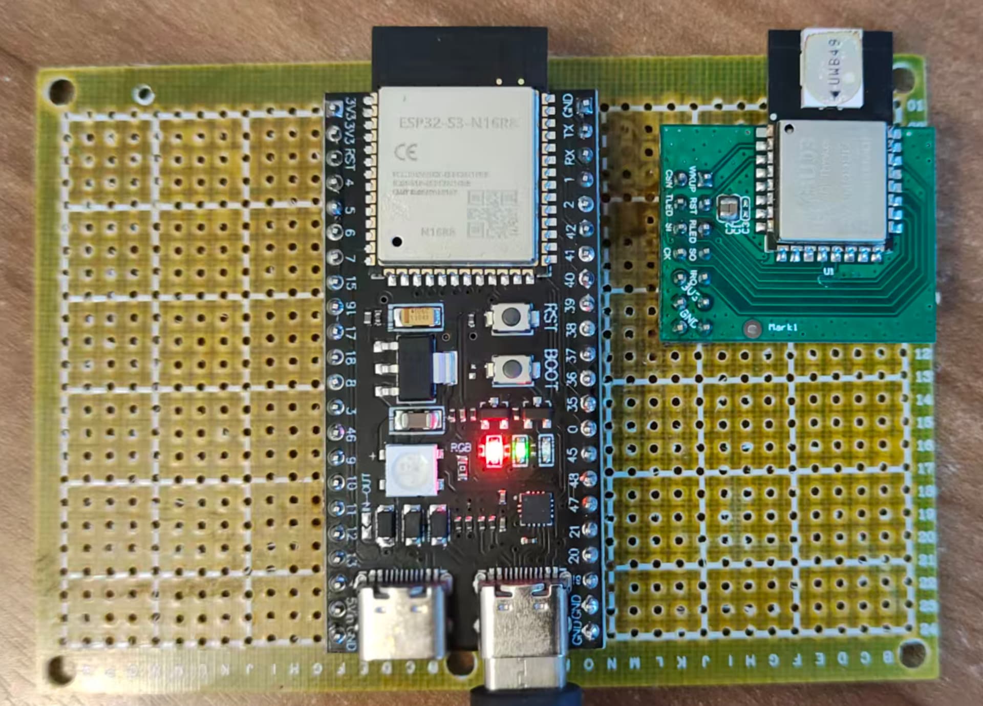
In this article, we use the Qorvo DW3000 UWB chip (Qorvo acquired Decawave). The DW3000’s internal timer is 40 bits wide, with a clock frequency of approximately 63.8976 GHz (meaning each tick has a time interval of approximately 15.65 picoseconds, corresponding to a spatial resolution of approximately 4.7 millimeters).

The 40-bit timer has a full-scale range of approximately 2^40 * 15.65 (ps) = 17.2 (seconds). This means the timer overflows (wraps around to zero) approximately every 17.2 seconds. This overflow must be carefully handled in software — if two timestamps are on opposite sides of the overflow point, a simple subtraction will yield an incorrect result. We will discuss how to handle this in detail in later chapters.

Tip: Although the 15.65ps timer resolution is extremely fine, this does not mean DW3000’s actual ranging accuracy is 4.7mm. Practical accuracy is affected by many factors, including antenna delay, multipath effects, clock stability, and more. Under ideal conditions (unobstructed, line-of-sight), DW3000 typically achieves ranging accuracy within ±10cm.

1.2 TDOA Positioning Principle

What is TDOA?

TDOA stands for Time Difference of Arrival. As the name suggests, it calculates the emitter’s position by measuring the time differences of the same signal arriving at different receiving points.

In fact, the GPS/BeiDou satellite navigation systems we use daily are essentially a form of TDOA — the GPS chip in your phone receives signals from multiple satellites and calculates the phone’s position based on the time differences of these signals’ arrivals. GPS/BeiDou use Downlink TDOA positioning, where the device being positioned calculates its own coordinates.

TDOA vs TOA/TWR:

Often mentioned alongside TDOA are TOA (Time of Arrival) and TWR (Two-Way Ranging). TOA calculates distance by measuring the absolute flight time from transmission to arrival, requiring strict clock synchronization between transmitter and receiver. TWR measures distance through two (or more) round-trip communications between sender and receiver, requiring no clock synchronization, but each ranging measurement requires bidirectional air-interface resources. TDOA only requires a unidirectional signal plus the time difference between receivers, without needing to know the absolute transmission time, making it more flexible and better suited for large-scale deployments.

Explaining the Principle Using Uplink TDOA

Downlink TDOA is more complex to explain, so let’s first use Uplink TDOA as an example to illustrate the TDOA positioning principle.

In Uplink TDOA, the Tag (the device to be positioned) transmits a UWB positioning signal, and nearby Anchors (base stations/reference points) receive this signal. Radio waves travel through air at the speed of light (approximately 3 * 10^8 m/s). Since each Anchor is at a different distance from the Tag, each Anchor receives the signal at a slightly different time — the farther Anchor receives it later, and the closer one receives it earlier.

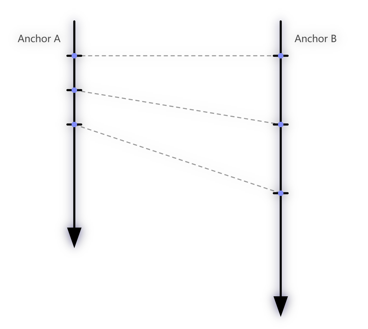
For example, consider two Anchors A and B, where Anchor A is farther from the Tag and Anchor B is closer. The two Anchors receive the signal at different times. Subtracting these two timestamps gives the Time Difference of Arrival of the Tag’s signal at Anchors A/B. Multiplying this time difference by the speed of light yields the distance difference between the Tag and the two Anchors.

The Mathematical Principle — Hyperbolic Positioning

From a mathematical perspective, let’s say the distance difference between the Tag and Anchors A/B is dAB. Using A and B as the two foci, we can draw a hyperbola on a plane (or a hyperboloid in 3D space). Every point on this hyperbola has the same distance difference dAB to A and B. In other words, the Tag must be located somewhere on this hyperbola.

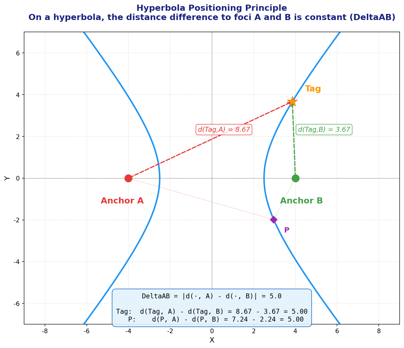
With just one hyperbola, we only know the Tag is somewhere on the curve — we cannot determine the exact coordinates. If we add another Anchor C, we get another independent hyperbola (e.g., with A/C as foci and distance difference dAC). The intersection of two hyperbolas (typically one or two points) gives the Tag’s candidate position(s).

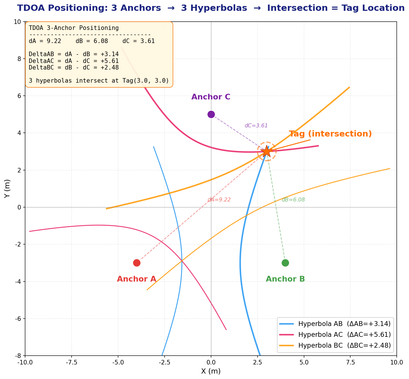
A Note on the Number of Independent Equations:

Some readers may wonder: don’t 3 Anchors give 3 pairs (AB, AC, BC)? Why only 2 independent hyperbolas? The reason is that dBC = dAC - dAB — the third time difference can be derived from the first two and provides no new independent information. In general, n Anchors produce n-1 independent TDOA equations.

2D positioning (solving for x, y): requires at least 3 Anchors (2 independent equations for 2 unknowns)

3D positioning (solving for x, y, z): requires at least 4 Anchors (3 independent equations for 3 unknowns)

Note: The hyperbola diagrams above are 2D illustrations to help you intuitively understand the positioning principle. In reality, our space is three-dimensional, and mathematically we’re dealing with hyperboloids. Three hyperboloids intersect along a curve (not at a point), so 3D positioning requires at least 4 Anchors.

Handling the Z-Axis

Even if we only want 2D positioning (solving for x/y), Anchors are typically deployed at elevated positions (e.g., on the ceiling at 3–5 meters height), while Tags are at lower positions (e.g., worn on a person’s chest at about 1.5 meters). There is a significant height difference between Anchors and Tags. Ignoring this height difference and calculating purely in a 2D plane would introduce systematic distance errors. Therefore, coordinate calculations must still be performed in 3D space, but we can fix the Tag’s z coordinate as a constant (e.g., 150cm). This way, the unknowns are only x and y, but distance calculations still account for the true 3D distances.

Improving Accuracy with More Anchors

In practice, we typically deploy more Anchors than the minimum required. The additional Anchors provide redundant information (an over-determined system), which can be processed using methods like least squares to improve positioning accuracy and robustness.

For 3D positioning, the vertical distribution of Anchors also matters — you cannot mount all Anchors on the ceiling at the same height. If all Anchors are on the same horizontal plane, information in the z direction is extremely weak (GDOP diverges in the z direction). Some Anchors should be deployed at lower heights, roughly at the same level as the Tag or even lower.

The Concept of GDOP (Geometric Dilution of Precision):

Similar to GPS satellite positioning, the spatial geometric distribution of Anchors has a huge impact on positioning accuracy. If all Anchors are clustered in a small area, the hyperboloids are nearly parallel, and small timing measurement errors will cause enormous coordinate deviations — imagine two nearly parallel lines where a tiny angle change shifts the intersection point dramatically. Conversely, if Anchors are evenly distributed around the Tag (ideally surrounding it from multiple directions), positioning accuracy is much better.

This is the concept of GDOP (Geometric Dilution of Precision). GDOP is a dimensionless multiplier — the smaller the GDOP, the better the geometry, and the less the measurement error is amplified. When deploying Anchors, ensure their spatial distribution is uniform and avoid placing all Anchors in a line or clustering them in one corner.

Uplink TDOA Data Flow

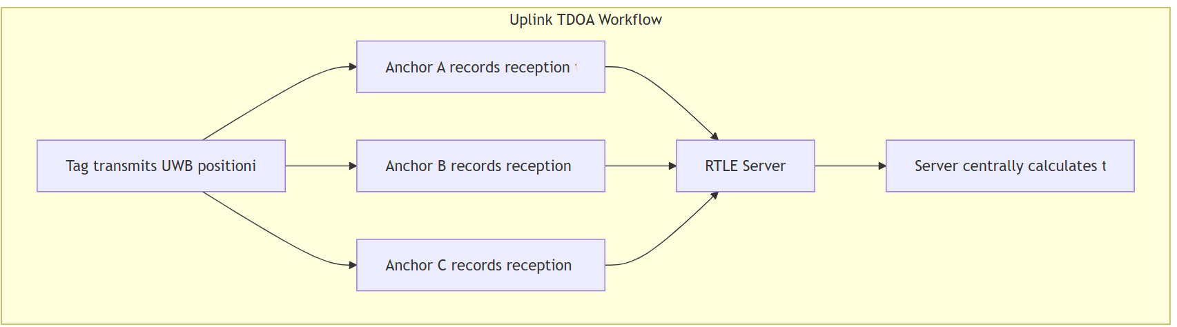
The process described above is the Uplink TDOA principle. The specific data flow is as follows:

The Tag transmits a UWB data packet
Multiple Anchors receive this packet and each records a reception timestamp
Each Anchor sends the packet content and its reception timestamp over a network (Ethernet/WiFi) to the RTLE (Real-Time Location Engine) — positioning calculation software running on a server
The RTLE calculates the Tag’s position based on the timestamp differences across Anchors and the known Anchor coordinates

Typically, Uplink TDOA coordinate calculations are performed centrally by the RTLE, and the Tag itself does not participate in the computation.

Clock Synchronization — The Foundation of TDOA Systems

As we’ve established, coordinate calculation requires knowing the time differences of signal reception across Anchors. The Tag sends its positioning packet at one definite moment, but the timestamps recorded by each Anchor when they receive this packet must be based on the same time reference to be meaningfully compared and subtracted.

Why is Clock Synchronization Necessary?

Under normal circumstances, each Anchor’s UWB chip uses its own independent crystal oscillator to drive its internal timer. Due to manufacturing tolerances (crystal frequency tolerance, load capacitance variation, chip internal circuit differences) and environmental changes during operation (temperature, voltage, and humidity fluctuations), each UWB chip’s internal counter runs at a slightly different frequency.

Even if calibrated at the factory, after some runtime the timestamp discrepancies between different devices will grow increasingly large. UWB positioning demands nanosecond-level timing accuracy (1ns ≈ 30cm), so even minuscule frequency deviations (on the order of parts per million, or ppm) will accumulate to unacceptable levels in very short periods.

A Real-Life Analogy: Everyone has experienced this — a wall clock and a wristwatch, even if set to the same time on the same day, will show a discrepancy of several seconds or even tens of seconds after just a few days. UWB chip crystal oscillators behave the same way.

Let’s do a quick calculation: Assume two Anchors have a crystal frequency difference of 5ppm (very common for ordinary crystals). The UWB chip’s reference frequency is approximately 499.2MHz. A 5ppm deviation means the frequency difference between the two chips is approximately 499.2 MHz * 5 * 10^(-6) = 2.496 kHz. The accumulated time offset per second is approximately 5 * 10^(-6) s = 5 us. A 5 microsecond offset corresponds to a distance error of 5 * 10^(-6) * 3 * 10^(8) = 1500 meters! In other words, without clock synchronization, after just 1 second, the timing discrepancy between two Anchors is enough to cause a 1,500-meter distance error.

Another vivid example: In a running race, if each athlete is timed with a separate stopwatch, but each stopwatch runs at a slightly different speed — even if they all read “10.00 seconds,” the fast stopwatch hasn’t actually measured a full 10 seconds, while the slow one has measured more. These results obviously can’t be fairly compared.

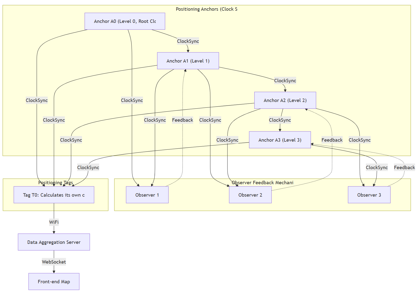
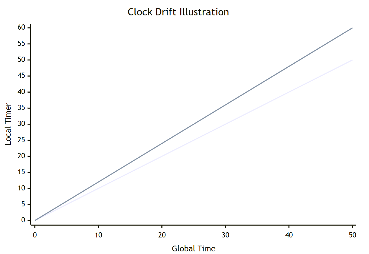
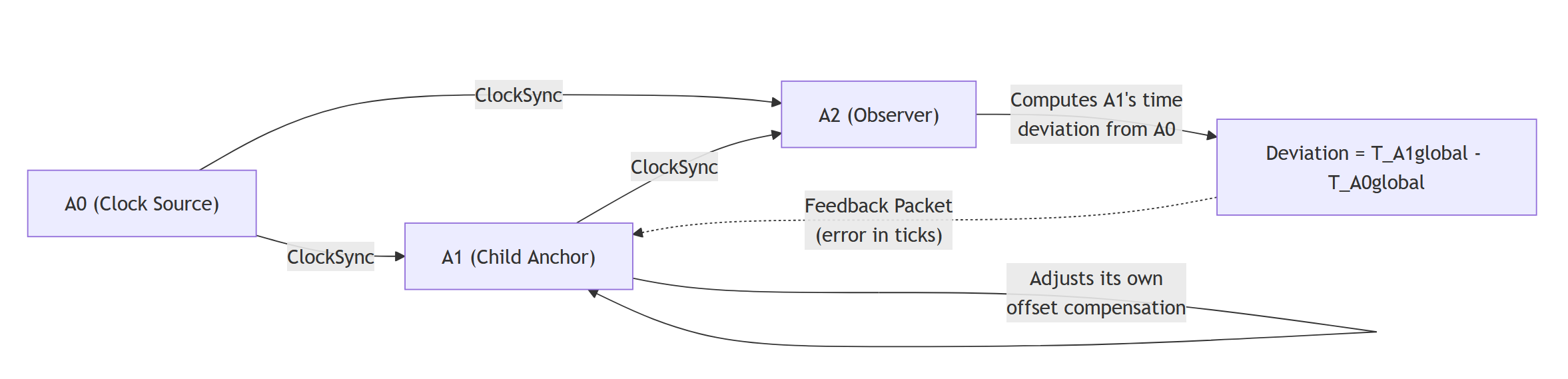
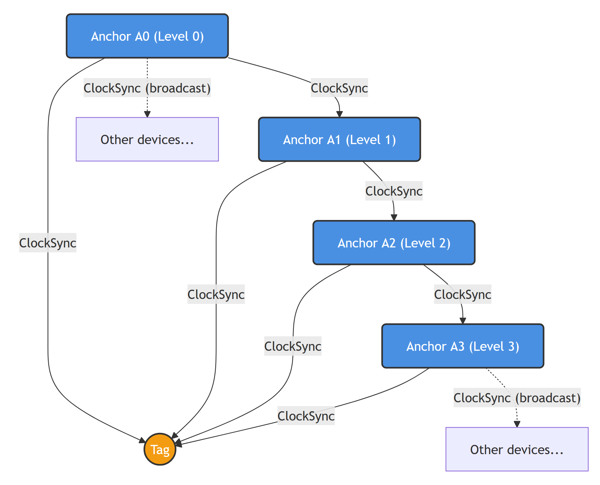
The Basic Approach to Clock Synchronization

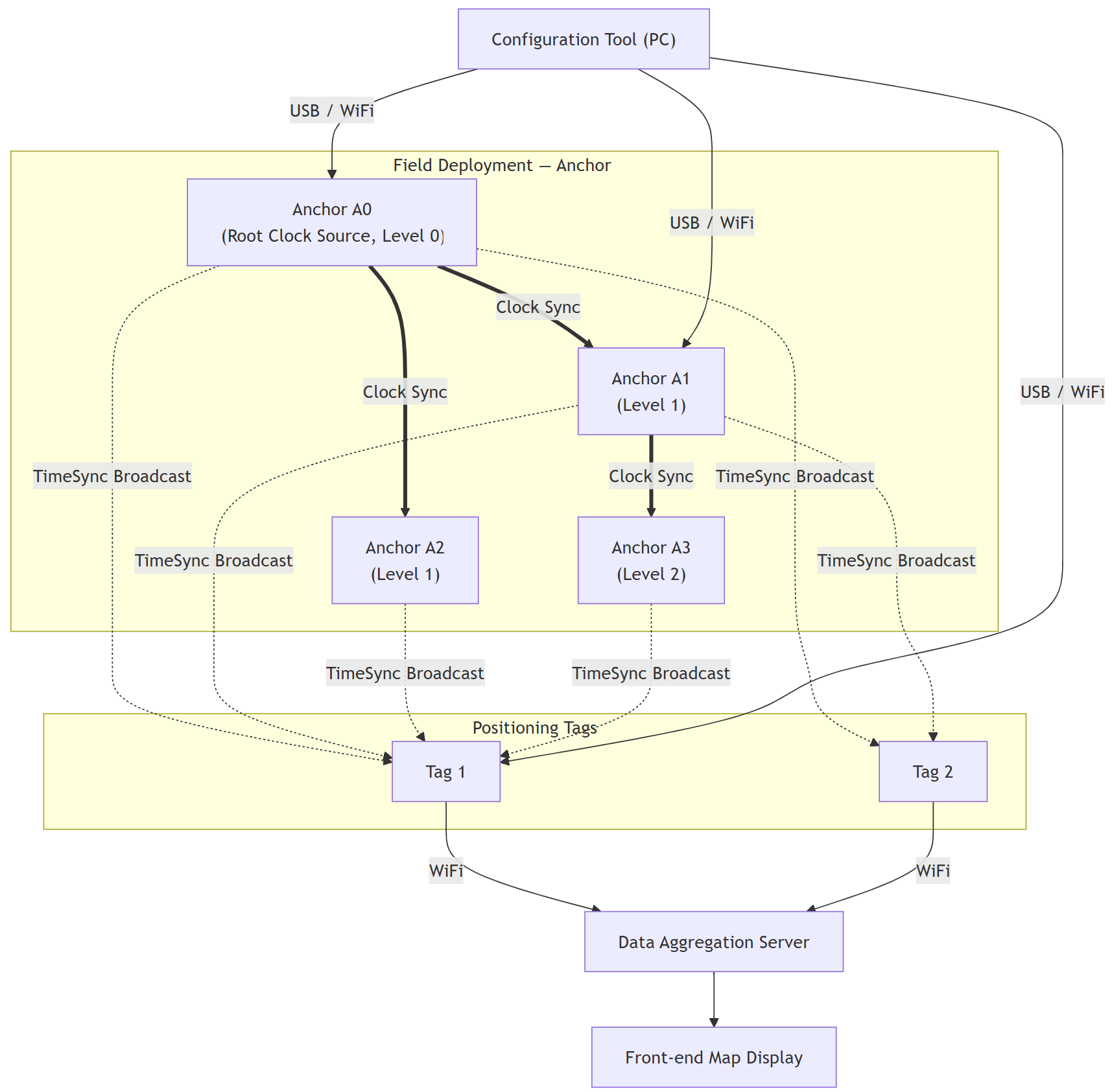
Typically, one Anchor is designated as the Root Clock Source (also called the reference Anchor). It periodically transmits clock synchronization signals (TimeSync packets). Other Anchors receive these synchronization signals and use algorithms to internally maintain a “Global Time” consistent with the clock source. We call this process Clock Synchronization.

Strictly speaking, “clock synchronization” and “time synchronization” are different concepts — “clock synchronization” focuses on making device clock frequencies consistent (frequency synchronization), while “time synchronization” focuses on making time values consistent (phase synchronization). However, in this article we don’t distinguish rigorously — our goal is for each Anchor to maintain an accurate Global Time so that our software can convert between any Anchor’s/Tag’s Local Time and Global Time.

Local Time vs Global Time:

Local Time: The raw reading of a specific UWB chip’s internal timer. Each chip has its own independent local time.

Global Time: A unified time based on the clock source. Through clock synchronization parameters, any Anchor/Tag can convert its local time to Global Time.

Downlink TDOA

As we know, in Uplink TDOA, the Tag transmits the positioning signal and all Anchors receive it. We simply subtract the Anchors’ Global Time timestamps of receiving the signal to get the time differences.

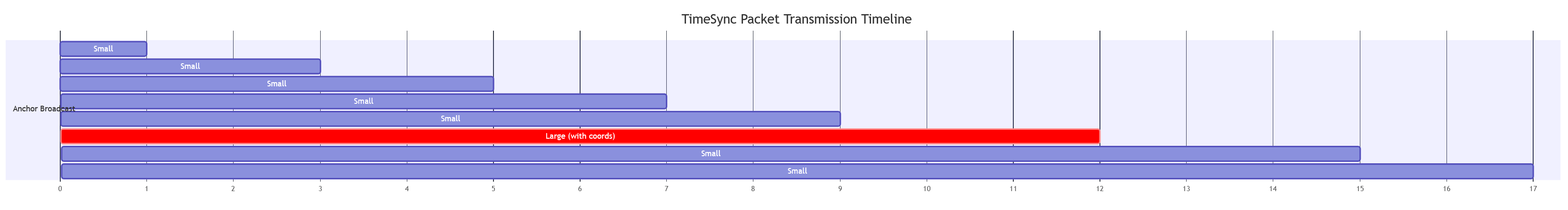
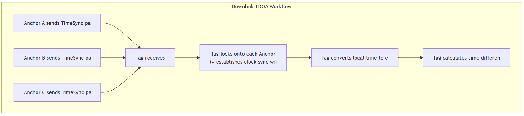
Downlink TDOA is more complex: each Anchor actively transmits positioning packets (called TimeSync packets), and the Tag records the timestamps of receiving these packets, then “figures out” the time differences.

Why Can’t We Simply Subtract?

The reason is that a Tag’s UWB receiver typically has only one channel and can only receive one signal at a time. Since each Anchor transmits its TimeSync packet at a different time, the Tag naturally receives them at different times. Because the transmission times differ, we cannot simply subtract the Tag’s local timestamps of receiving each packet to get the time difference — these timestamp differences contain both the desired distance-difference information and the Anchor transmission time differences, all mixed together inseparably.

Tag “Locking” onto Anchors

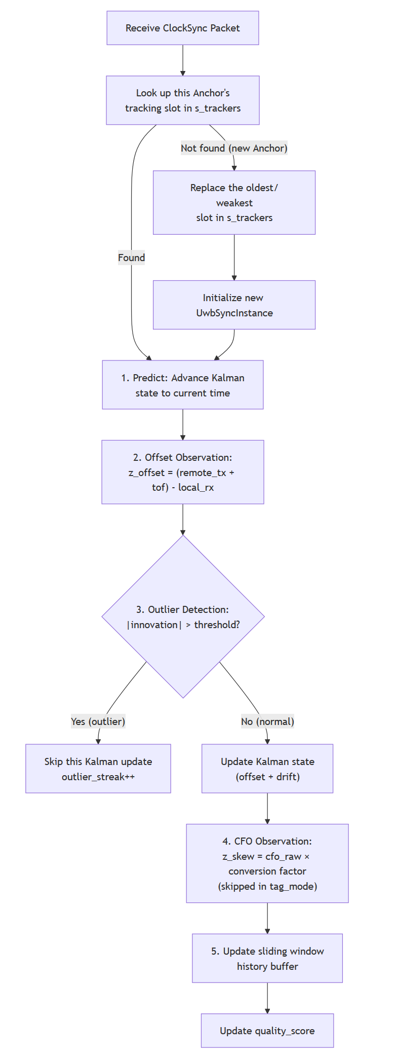
To solve this problem, the Tag needs to perform a locking operation on each Anchor. “Locking” is essentially the Tag performing clock synchronization with a specific Anchor. Through locking, the Tag maintains “Global Time” information derived from that Anchor internally. This enables the Tag to convert its local time to that Anchor’s corresponding Global Time at any moment.

More precisely, by continuously receiving TimeSync packets from a specific Anchor, the Tag estimates the frequency offset (skew) and time offset between its own local clock and that Anchor’s global clock. With these two parameters, the Tag can convert any local timestamp to that Anchor’s corresponding Global Time.

Once the Tag has locked onto multiple Anchors (e.g., 4), for any specific local timestamp tlocal, the Tag can convert it to 4 separate Global Times _ t(G,1), t(G,2), t(G,3), t(G,4) _ corresponding to each Anchor. Since the Tag’s distance to each Anchor differs, these 4 Global Times will differ — subtracting them pairwise yields the Time Difference of Arrival (TDOA).

Why Does This Method Successfully Isolate the Distance Difference?

The key lies in the physical meaning of “Global Time.” Imagine the Tag asking: “If all Anchors simultaneously sent signals to me right now, how long would each signal take to arrive?” Through clock synchronization parameters, the Tag can map its local time to each Anchor’s Global Time. Due to different distances, the differences between these mapped times precisely reflect the flight time differences caused by distance differences.

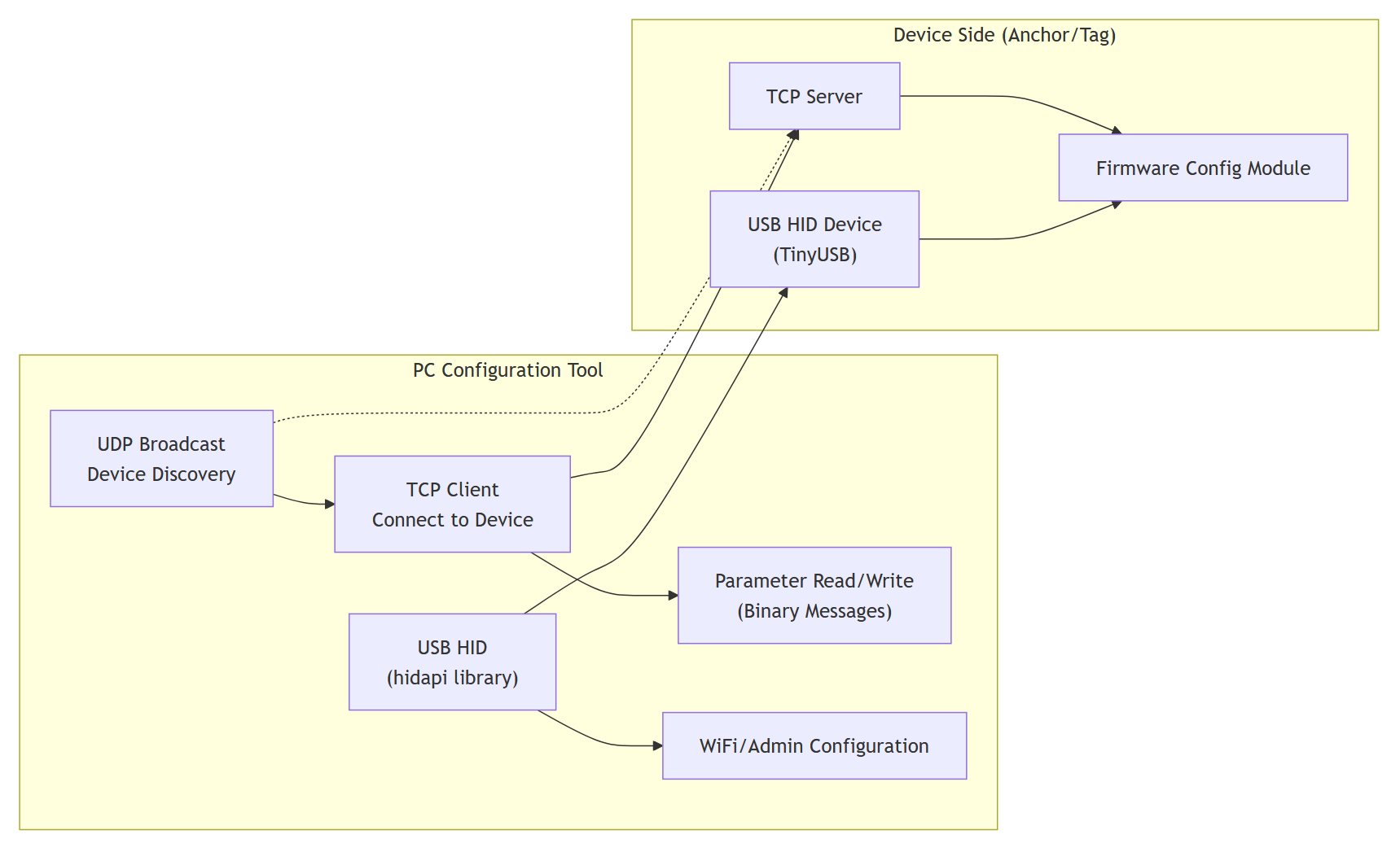
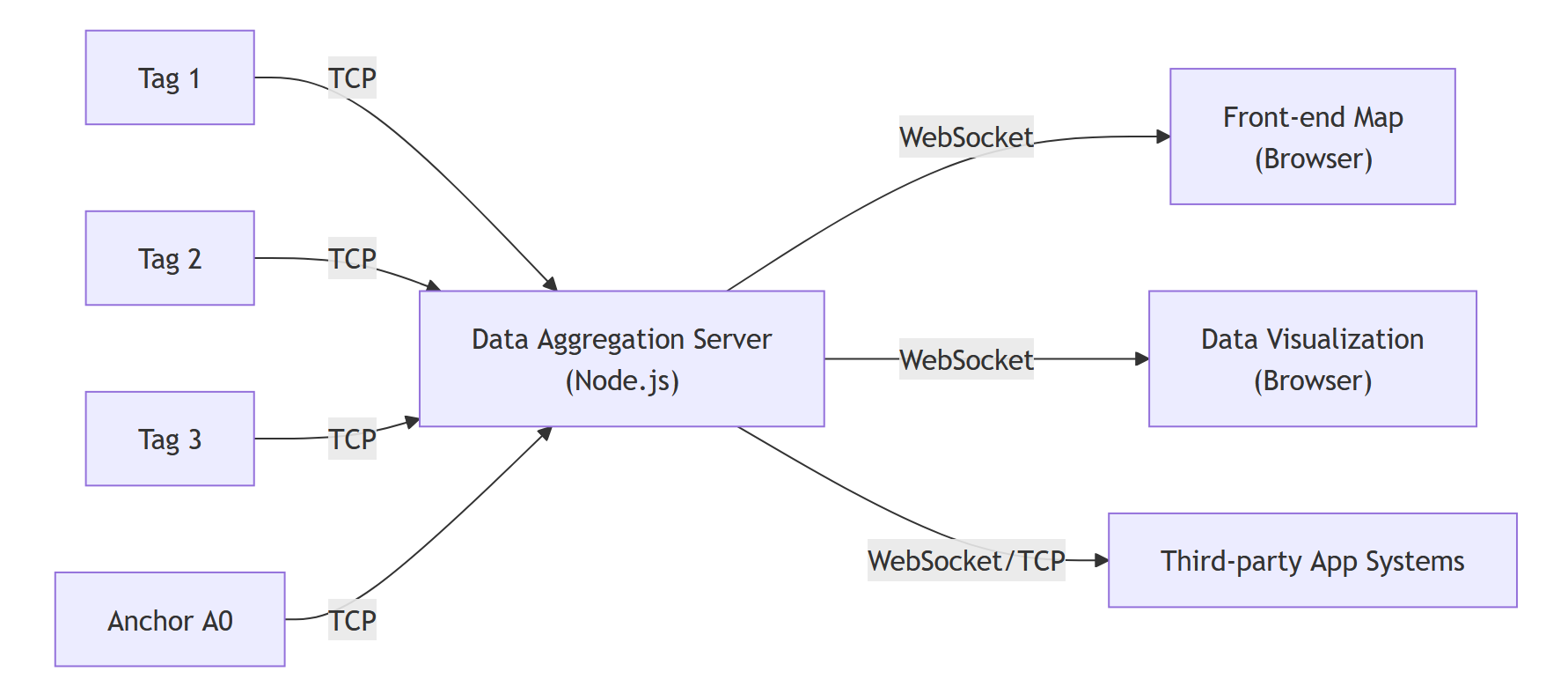
The following flowchart compares the workflows of Uplink TDOA and Downlink TDOA:

We will explain “Clock Synchronization” and “Locking onto Anchors” in more detail in later chapters.

1.3 Uplink TDOA vs Downlink TDOA

The comparison between Uplink TDOA and Downlink TDOA is shown in the following table:

Comparison Item	Uplink TDOA	Downlink TDOA
Positioning signal sender	Tag transmits	Anchors transmit
Positioning signal receiver	Anchors receive	Tag receives
Clock sync occurs between	Anchors only	Anchors + Tag-to-Anchor
Clock sync precision req.	Moderate-high precision	Extremely high precision required
Coordinate calculation	Centralized on a dedicated server (RTLE)	Tag calculates locally (no server needed)
Tag power efficiency	Very power-efficient (sleeps, periodically wakes to transmit)	Higher power consumption (must stay in receive mode continuously)
Tag hardware cost	Very low (minimal functionality, only needs to transmit)	Higher (needs larger RAM and more capable MCU for calculations)
Infrastructure cost	Requires a dedicated server for the location engine	No dedicated positioning server needed; lower total cost
System capacity/scalability	Tag contention increases with count; needs TDMA/FDMA management	Anchors broadcast; Tag count has no theoretical limit (receive-only)
Privacy	Coordinates calculated on server; Tag cannot keep its location private	Coordinates calculated locally on Tag; Tag can choose not to report

Supplementary Note — System Capacity:

In Uplink TDOA, every Tag needs to transmit signals over the air. When the Tag count is high, the UWB channel becomes crowded, and packet collisions may occur. Complex TDMA (Time Division Multiple Access) or FDMA (Frequency Division Multiple Access) mechanisms are needed to manage air-interface resources — for example, assigning each Tag a specific transmission time slot, or having Tags use random backoff algorithms (similar to WiFi’s CSMA/CA). Even so, when the Tag count reaches hundreds or thousands, the system’s update rate and reliability will significantly degrade.

In Downlink TDOA, Anchors periodically broadcast TimeSync signals, and Tags only receive without transmitting. Therefore, the number of Tags has theoretically no upper limit — you can deploy any number of Tags in the same area without them interfering with each other. This is a very significant advantage of Downlink TDOA in large-scale deployment scenarios (such as large warehouses, stadiums, and shopping malls).

Supplementary Note — Privacy:

Downlink TDOA has another often-overlooked advantage: location privacy. Since coordinates are calculated locally on the Tag, the Tag can choose not to report its position to any server. This is important in certain privacy-sensitive application scenarios (such as military applications or personal tracking devices).

1.4 Technical Key Points of Downlink TDOA

Readers who have followed my previous article series should have a basic understanding of TDOA technology and know that clock synchronization and coordinate calculation are the two core technical challenges. Let’s now analyze what special technical requirements Downlink TDOA has in these areas.

1.4.1 Clock Synchronization — The Greatest Challenge of Downlink TDOA

Downlink TDOA demands significantly higher clock synchronization precision than Uplink TDOA. This is the most critical challenge in Downlink TDOA system design. Here’s why:

In Uplink TDOA, all Anchors receive the same signal transmitted by the same Tag at the same moment. Although each Anchor’s timestamp is based on its own local clock, the clock synchronization error only affects the computation of timestamp differences — and this error is “common-mode” to some extent, partially cancellable through differential computation.

In Downlink TDOA, however, each Anchor transmits signals at different times, and the Tag must use clock synchronization parameters to convert its local timestamps (recorded at different reception times) into each Anchor’s Global Time. Clock synchronization errors are directly and fully superimposed onto the final time differences. For example:

If the clock synchronization error between Anchors is 1 nanosecond, this translates to approximately 30 centimeters of positioning error
If the sync error is 3 nanoseconds, the error approaches 1 meter
If the sync error is 10 nanoseconds, the system becomes essentially unusable

Therefore, Downlink TDOA typically requires sub-nanosecond (<1ns) clock synchronization precision.

1.4.2 Multipath Propagation and First Path Detection

We know that during radio wave propagation, obstructions and interference can prevent the receiver from getting a signal, or the received signal may not come from the First Path — the direct line-of-sight propagation path.

What is Multipath Propagation?

Theoretically, radio waves travel in straight lines (this is the physical basis for radio-based positioning). In practice, however, radio waves exhibit multipath propagation. This means that the signal from transmitter to receiver may travel along many paths:

First Path (Line-of-Sight, LOS): Direct straight-line transmission, the shortest path, arriving earliest — this is the only path we want for positioning
Reflected paths: Signals bouncing off walls, ceilings, and floors before reaching the receiver
Diffracted paths: Signals bending around the edges of obstacles to reach the receiver
Scattered paths: Signals encountering rough surfaces or small objects and scattering in multiple directions

Only the First Path corresponds to the true straight-line distance. All other paths have longer transmission distances and later arrival times.

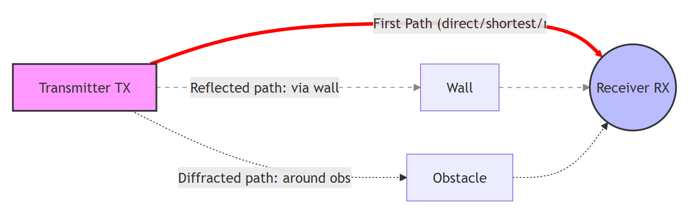
Legend:

Red solid line: The First Path from transmitter to receiver — shortest path, most accurate timing
Gray dashed lines: Multipath signals reflected/diffracted off walls and objects — longer paths, later arrivals

BD8NCF · May 15, 2026, 3:51pm

The Problem of First Path Being “Swallowed”

Logically, the first signal the receiver detects should be from the First Path — since it’s the shortest distance, it should arrive first. However, the reality is more complicated:

First Path may be partially obstructed (NLOS): If there’s an obstacle between the transmitter and receiver (such as a wall, human body, or metal equipment), the First Path signal will be attenuated or completely blocked. This is called NLOS (Non-Line-of-Sight).
Strong multipath signals suppressing the weak First Path: Even if the First Path signal isn’t completely blocked, it may be weakened significantly. Meanwhile, certain reflected paths (e.g., reflected off large metal surfaces) may actually be stronger.
AGC effects: Receivers typically have an AGC (Automatic Gain Control) circuit. When received signals are too weak, AGC automatically increases the amplification gain; when signals are too strong, AGC reduces the gain. AGC’s role is to adjust the signal amplitude to the ADC’s (Analog-to-Digital Converter) optimal input range.

The problem is: if a stronger multipath signal triggers AGC adjustment first (reducing gain), the subsequently arriving weak First Path signal may be “drowned” in noise. Conversely, if AGC is at high gain when a very strong multipath signal arrives, ADC saturation may occur.

Radio analogy: If you’ve used a shortwave radio, you may have noticed — when tuning to a frequency with no signal, background noise gradually increases (AGC is trying hard to amplify); when tuning to a frequency with a signal, background noise decreases or disappears (AGC has reduced the gain). UWB receiver AGC works similarly.

LDE — Preamble Detection and First Path Extraction

The chip identifies data packets through the preamble. The structure of a UWB data packet is roughly:

┌──────────────┬───────────────┬──────────┬──────────────┐
│  Preamble    │     SFD       │   PHR    │   Payload    │
│              │ (Start Frame  │ (PHY     │              │
│              │  Delimiter)   │  Header) │              │
└──────────────┴───────────────┴──────────┴──────────────┘

The receiver continuously monitors incoming wireless signals. When it determines that the received signal matches the expected preamble pattern (a specific pseudo-random sequence), it knows a complete data packet is coming. The preamble is repeated multiple times (DW3000 supports configurable preamble lengths from 16 to 4096 symbols) to ensure the receiver can correctly identify it under various signal-to-noise ratio conditions.

During preamble detection, the chip’s LDE (Leading Edge Detection) algorithm is responsible for precisely pinpointing the First Path’s arrival time within the received signal. Due to multipath effects, the received waveform is a superposition of multiple delayed signal copies. LDE must distinguish the earliest arriving pulse — the leading edge — from among these overlapping signals.

When the signal is particularly weak, or particularly strong and approaching saturation, LDE may deviate in extracting the First Path, causing the receiver’s reported “reception timestamp” to be inaccurate. This deviation is non-negligible in high-precision clock synchronization.

What is CFO (Carrier Frequency Offset)?

When the DW3000 chip receives a data packet, its internal carrier recovery loop estimates the Carrier Frequency Offset (CFO). This value reflects the frequency difference between the transmitter and receiver crystal oscillators.

The physical essence of CFO is the frequency difference between two crystal oscillators, typically expressed in ppm (parts per million) or ppb (parts per billion). CFO can serve as auxiliary information to determine clock drift rate (drift/skew) and can also help identify abnormal reception events (if a packet’s CFO differs significantly from historical values, the packet may have been affected by interference or may not be from the First Path). We will use this value in later chapters when discussing advanced clock synchronization.

Practical Deployment Considerations

In practical deployments, Anchor installation positions are carefully planned — typically installed in open locations with clear line-of-sight between them. Therefore, inter-Anchor communication usually receives the First Path signal correctly. However, temporary obstructions (e.g., someone placing a metal cabinet in the signal path) or transient interference may still cause the receiver to detect a non-First Path signal. In such cases, we need to design anomaly detection and filtering mechanisms in software — checking signal quality indicators (such as First Path power, received signal power, CFO, etc.) to determine whether a particular reception is trustworthy, and discarding untrustworthy data directly.

1.4.3 Distance Compensation in Clock Synchronization

During clock synchronization, there’s another important issue to address: the clock source transmits a TimeSync signal, and other Anchors receive it — but the signal needs time to travel from the clock source to each Anchor! This flight time equals their distance divided by the speed of light.

In Uplink TDOA, this distance offset can be uniformly compensated in the RTLE positioning engine — since the RTLE knows all Anchor coordinates and can factor this into its calculations.

In Downlink TDOA, however, there is no centralized positioning engine. The distance offset between the clock source and each Anchor must be compensated during the clock synchronization phase itself. This means that after receiving the clock synchronization signal, each Anchor needs to subtract the signal’s flight time based on its known distance to the clock source to obtain the accurate Global Time.

This requires that each Anchor’s coordinates and the clock source’s coordinates be pre-configured in every Anchor’s firmware during system setup. Each Anchor automatically calculates its distance to the clock source at startup and applies compensation during clock synchronization.

What does this mean for deployment? Every time you deploy or move an Anchor, you need to reconfigure the coordinate information. This adds deployment complexity, but it is essential for maintaining positioning accuracy.

1.5 System Planning

The overall architecture of the Downlink TDOA positioning system is illustrated below:

Clock Synchronization Hierarchy (Levels)

In the diagram above, you may have noticed the “Level 0”, “Level 1”, “Level 2” labels after each Anchor. This represents the clock synchronization hierarchy:

Level 0: The Root Clock Source — the time reference for the entire system. There is only one Level 0 Anchor in the entire positioning area.
Level 1: Anchors that directly obtain clock synchronization from Level 0. They can “hear” the TimeSync signals transmitted by Level 0.
Level 2: Anchors that cannot directly hear Level 0’s signals, and instead obtain clock synchronization from a Level 1 Anchor.
And so on — there can be Level 3, Level 4, etc.

Why is a multi-level structure needed? Because UWB signal range is limited (DW3000 typically has an effective indoor communication range of 20–40 meters, depending on transmit power, antenna gain, and environmental obstructions). If the positioning area is large (e.g., a warehouse of several thousand square meters), distant Anchors may not be able to receive Level 0’s signal at all. Through multi-level cascading, the clock synchronization signal can be “relayed” to more distant Anchors.

Caution: Each additional level accumulates an extra layer of synchronization error. Therefore, the number of levels should not be excessive (typically recommended not to exceed 2–3 levels). When planning the system, the Root Clock Source should be placed as close to the center of the positioning area as possible to minimize the number of required levels.

System Components

Anchor Network: Several Anchor hardware devices are deployed at the positioning site. Anchors maintain clock synchronization via UWB and connect to the LAN via WiFi (for configuration management and status monitoring).
Tags (Positioning Tags): Fixed or mobile devices to be positioned. Tags receive TimeSync broadcast packets from Anchors and calculate their own coordinates locally.
Tag Application Modes: A Tag can be a standalone offline application (e.g., a handheld device with a screen that displays its own coordinates), or it can connect to WiFi and send coordinate data to an application server.
PC Configuration Tool: Communicates with devices via USB or WiFi to configure various parameters for Anchors and Tags (such as coordinates, WiFi SSID/Password, clock sync hierarchy level, UWB channel parameters, etc.).
Data Aggregation Server: To facilitate application development, a server-side program can be written to collect coordinate information from all Tags and provide a unified interface for application systems (e.g., via WebSocket or MQTT push to the front-end).
Front-end Map Application: For convenient deployment and debugging, a simple front-end map application can show each Tag’s real-time position on a floor plan.

Development Task List

Based on the above planning, the major development tasks are:

Anchor hardware design — Including ESP32-S3 + DW3000 + WiFi antenna + UWB antenna + power supply circuit
Tag hardware design — Including ESP32-S3 + DW3000 + lithium battery power supply/charging circuit
Anchor firmware — Clock synchronization, TimeSync broadcasting, WiFi connectivity, configuration management
Tag firmware — Anchor locking, clock synchronization, TDOA coordinate calculation, WiFi connectivity
PC configuration tool — USB communication + WiFi communication, parameter configuration interface
Data aggregation backend — Collecting coordinate data from multiple Tags, providing API interfaces
Map display front-end — Loading floor plans, real-time Tag position display

2. Hardware Selection and Design

2.1 Component Selection

2.1.1 MCU Selection

Readers who have followed my previous articles know that I mostly used STM32 series MCUs as the main controller in my earlier embedded system designs. However, I later shifted toward the ESP32 series. My reasons for moving away from STM32 include:

Price volatility and supply instability. I experienced several STM32 price surges (particularly severe during the 2020–2021 chip shortage, when some models saw prices increase by 10x or more). Domestic STM32-compatible chips (such as GD32, AT32) are plentiful, but they also raise their prices whenever STM32 prices rise.
Domestic alternatives still need time to mature. Documentation completeness and technical support responsiveness still fall short. As a side note, many domestic chip manufacturers tend to be secretive — even downloading a datasheet may require signing an NDA. When you encounter technical issues, the manufacturer often provides as little information as possible, like squeezing toothpaste from a tube, leaving developers in a very passive position.
Limited resources on STM32. STM32 targets traditional industrial control applications. Reasonably priced models (like STM32F1/F4) have tight RAM/Flash resources (the F103 has only 20KB RAM), while resource-rich models (like the STM32H7 series) come at premium prices.

For this project, we chose the ESP32-S3. It addresses each of the above concerns:

Feature	STM32 (Common Models)	ESP32-S3
Price stability	Volatile	Stable, good value
RAM	20KB–1MB (model/price dependent)	512KB on-chip + up to 8MB external PSRAM
Flash	64KB–2MB	Up to 16MB external SPI Flash
CPU	Single-core 72–480MHz (Cortex-M series)	Dual-core 240MHz Xtensa LX7
WiFi	None (requires external module)	Built-in WiFi 4 (802.11 b/g/n)
Bluetooth	None (requires external module)	Built-in BLE 5.0
USB	Some models have USB OTG	Built-in USB OTG (native USB)
Documentation/Community	Rich	Very rich (ESP-IDF official docs + community)

However, ESP32 also has some issues to be aware of (such as floating-point operation restrictions in ISRs and byte alignment exceptions discussed later) — I will cover these in detail in subsequent sections.

When selecting within the ESP32 family, there are many models to choose from (ESP32 Classic, ESP32-S2, ESP32-S3, ESP32-C3, ESP32-C6, ESP32-H2, etc.). I initially planned to use the classic ESP32 but decided on the ESP32-S3 after careful comparison.

Our core MCU requirements were:

WiFi. If the MCU has built-in WiFi, there’s no need for an external WiFi chip/module, saving cost, PCB area, and firmware complexity. All ESP32 variants except ESP32-H2 include WiFi.
USB provisioning. We need some way to tell the firmware the WiFi SSID and password. Common approaches include:
- WiFi provisioning protocols (SmartConfig, SoftAP mode) — requires a smartphone app
- Bluetooth provisioning — also requires a smartphone app
- USB provisioning — only requires a PC configuration tool
I prefer USB for WiFi provisioning (the PC configuration tool sends WiFi credentials directly), eliminating the need to develop and maintain a smartphone app. This means the MCU must support native USB (USB OTG). Within the ESP32 family, ESP32-S2 and ESP32-S3 support native USB.
Computing power. The ESP32 family includes both single-core and dual-core MCUs. Since the Tag needs to perform coordinate calculations (involving matrix operations and numerical iterations), dual-core is preferred — one core handles UWB data reception and clock synchronization while the other handles coordinate calculation and WiFi communication, without blocking each other. The classic ESP32 and ESP32-S3 are dual-core.
Stability and ecosystem. Some ESP32 models use RISC-V cores (ESP32-C3, C6, H2). While the RISC-V architecture is very promising, its toolchain and ecosystem are slightly less mature compared to the well-proven Xtensa instruction set. From a conservative and stability standpoint, choosing an Xtensa-core MCU is more reassuring.

Considering all these requirements, the final choice was ESP32-S3.

2.1.2 UWB Chip Selection

I previously used the Decawave DW1000 and was quite familiar with its performance and driver interface. However, due to China’s radio spectrum regulation requirements, the frequency bands supported by DW1000 are not permitted for use in China. Currently, the only viable option from the Decawave/Qorvo lineage is the DW3000.

DW1000 vs DW3000 Frequency Band Differences:

The DW1000 primarily operates on Channels 1–7 (center frequencies approximately 3.5GHz–6.5GHz), and several lower-frequency channels (particularly Channels 1–4, center frequencies around 3.5–4.5GHz) are not approved for UWB use in China. The DW3000 supports Channel 5 (center frequency 6489.6MHz) and Channel 9 (center frequency 7987.2MHz), of which Channel 9 is permitted under China’s UWB regulations.

If your product needs to be sold in the Chinese market, ensure you use Channel 9 and comply with the relevant technical requirements from the national radio administration (including transmit power spectral density limits, etc.).

I also evaluated UWB chips from other companies:

NXP: Their UWB chips (such as the Trimension series) are difficult to purchase on the open market, and technical documentation requires signing an NDA. NXP’s UWB product line appears to focus on smartphone/automotive large-customer scenarios (like digital car keys and secure payments) and is not particularly friendly to small-volume positioning system developers. Customer feedback suggests NXP primarily promotes TWR (Two-Way Ranging) mode rather than TDOA, which doesn’t align with our technical approach.
A Domestic Chinese UWB Chip: Positioned as a DW3000 competitor, it’s an SoC with an integrated Cortex-M0 core, supporting 4 antennas and up to 31Mbps data rates — very feature-rich. However, the manufacturer’s technical support for small customers is inadequate, and even the datasheet requires an NDA. For positioning system development that requires register-level debugging, the lack of publicly available technical documentation is a critical issue.

Therefore, the final choice was Qorvo DW3000. In the UWB positioning field, the DW3000 currently has the most complete documentation, the most active community, and the best technical support available.

DW3000 Driver Considerations

Similar to the DW1000, Qorvo provides a driver library that encapsulates low-level register operations (Driver/API). Perhaps to maintain some API compatibility with DW1000, most function names remain similar.

But don’t be misled by the function names — DW3000’s register layout differs significantly from DW1000, and there are substantial functional differences (e.g., DW3000 adds STS — Scrambled Timestamp Sequence for secure ranging; data rates support up to 6.8Mbps; preamble configuration options have also changed). Even with DW1000 programming experience, you must carefully study the DW3000 User Manual.

The DW3000 driver includes an additional Platform Abstraction Layer (PAL) for cross-platform compatibility. This causes some unused feature functions to be compiled and linked into the firmware, increasing binary size. For MCUs with tight RAM/Flash, you may need to trim the DW3000 driver (commenting out unneeded functions, removing unused feature code). However, for the ESP32-S3, Flash and RAM are typically plentiful, so this is not a major concern.

2.1.3 Power Supply

Power supply design is a critical aspect of any embedded product, directly affecting system stability, battery life, and thermal management.

Anchor Power Supply

In the previous Uplink TDOA project, I used PoE (Power over Ethernet) for Anchor power — a single Ethernet cable handled both data and power, making deployment very convenient.

For the new project, since we switched from Ethernet to WiFi, PoE is no longer applicable. Anchors now use the following power options:

USB power (5V): Powered via a USB Type-C connector, convenient for use with power banks or USB adapters
DC 12V power: Powered via a DC power jack, suitable for permanent fixed installations (using a 12V switching power adapter)

Some Anchor variants also include a built-in lithium battery for deployment in locations without mains power. These can be periodically swapped out or removed for charging and then reinstalled.

Tag Power Supply and Charging

As a mobile device, the Tag requires lithium battery power. The charging approach continues from the previous project — USB charging or Qi wireless charging + lithium battery. However, the charging management IC received an important upgrade.

The previously used TP4057 is a linear charging IC: charging current flows directly from input to battery, and the heat dissipation equals the voltage difference times the charging current.

Pheat = (Vin - Vbatt) * Icharge

For example, when charging via 5V USB with a battery voltage of 3.8V, the voltage difference is 1.2V. At 500mA charging current:

Pheat = 1.2V * 0.5A = 0.6W

0.6W of heat generation is quite significant for a small device. Reducing the charging current to control heat means longer charging times; increasing the current makes the heat problem worse, potentially affecting lithium battery safety.

The new project uses the SLM6600 — a DC-DC switching charging IC. The heat generated by a DC-DC charger depends on conversion efficiency, not the input-output voltage difference. The SLM6600 achieves approximately 92% or higher charging efficiency under typical conditions:

Pheat = Pin * (1 - η) = (Vbatt * Icharge)/η * (1-η)

Under the same 3.8V/500mA charging conditions:

Pheat = (3.8 * 0.5)/0.92 * 0.08 = 0.17W

Only about one-third the heat of the linear charging approach. More importantly, we can safely increase the charging current to 1A or higher, dramatically shortening charging time while keeping heat manageable.

Linear vs DC-DC Charging — Quick Comparison:

Linear Charging (e.g., TP4057) DC-DC Charging (e.g., SLM6600)

Charging efficiency ~Vbatt/Vin (≈76% @ 3.8V/5V) ≈92%

Heat at 500mA charging ~0.6W ~0.17W

Can charging current be increased? Limited by thermal; hard to exceed 500mA Can safely increase to 1A or higher

External components Very few (1–2 resistors and capacitors) Requires inductor and freewheeling diode

PCB footprint Small Slightly larger (inductor takes space)

3.3V Regulation — Why a Buck-Boost Converter?

For lithium battery-powered devices, providing a stable 3.3V supply voltage is a challenging design decision. Lithium battery voltage ranges from 3.0V to 4.2V (4.2V fully charged, approximately 3.0V at discharge cutoff). To convert to 3.3V, there are two common approaches:

LDO (Low Dropout Regulator): Simple circuit, low cost, minimal output ripple, but low efficiency — when battery voltage is above 3.3V, excess energy is entirely wasted as heat; when battery voltage drops below 3.3V + LDO dropout voltage, the output voltage collapses and can no longer maintain 3.3V.
DC-DC switching regulator: High efficiency (typically 85%–95%), but more complex circuitry with switching ripple noise.

The previous project’s Tag used an XC6206P332 LDO for voltage conversion, which was adequate since that Tag had simple functionality and low current draw.

The new project uses the TI TPS63100 for voltage conversion. The TPS63100 has an input voltage range of 1.8V–5.5V, configurable output (set via external resistor divider; we set it to 3.3V), and a nominal output current of 1.5A.

The TPS63100’s most important feature is seamless buck-boost operation. When the lithium battery is fully charged at 4.2V (above 3.3V, requiring buck/step-down), and when discharged to 3.0V or lower (below 3.3V, requiring boost/step-up), the TPS63100 automatically switches between buck and boost modes across the entire battery operating voltage range, consistently providing a stable 3.3V output.

This feature is particularly important for UWB systems: the DW3000 chip draws significant peak current during UWB signal transmission (the DW3000 IC’s peak TX current is approximately 85mA at 3.3V; at the system level including antenna matching network and PCB trace losses, peak current can reach 100–140mA). If the supply voltage drops due to battery discharge and falls below DW3000’s minimum operating voltage (approximately 2.8V), it could cause DW3000 to reset or exhibit abnormal transmission power. The TPS63100 ensures that even as the battery voltage declines, the DW3000 still receives a stable 3.3V supply.

2.1.4 Network Connectivity

I deliberated for quite a long time over the networking approach. The previous Uplink TDOA project used Ethernet, with PoE conveniently solving the power issue. Ethernet’s advantages include:

Stable and reliable network connection, unaffected by wireless interference
Plug-and-play, no provisioning needed
Low latency, high bandwidth

But Ethernet’s disadvantages are also significant:

High cable material costs (each Cat5e cable from the PoE switch to the Anchor installation point may be tens of meters long)
High installation labor costs (especially when running cables and cable trays on ceilings, requiring professional installation teams)
Each installation point needs a pre-planned network port or cable tray

WiFi eliminates cables entirely, making deployment costs much lower — you only need to ensure WiFi AP coverage. However, WiFi has a provisioning problem: before connecting to an AP, each device needs to be configured with the WiFi SSID and Password.

Many WiFi IoT devices use smartphone apps (via WiFi SmartConfig broadcast or Bluetooth BLE) for provisioning. But this means developing and maintaining an additional mobile app (iOS + Android), adding system complexity.

To reduce system complexity, I use USB for network provisioning. The approach works as follows:

The device (Anchor or Tag) connects to a PC via USB Type-C
The PC configuration tool communicates with the device via USB CDC (virtual serial port)
Enter the WiFi SSID and Password in the configuration tool and click “Send”
The device receives the WiFi credentials, saves them to Flash (persistent across power cycles), and automatically connects to WiFi

Since we already need a PC configuration tool for setting various device parameters (coordinates, hierarchy level, channel parameters, etc.), having this tool also handle USB-based WiFi provisioning is the most natural and elegant solution — no need for a separate smartphone app, and no need to implement SoftAP or Bluetooth provisioning in the device firmware.

2.1.5 Fuel Gauge

In this project, some Anchors and Tags use lithium batteries, making battery management an important requirement — users need to know how much runtime remains and when charging is needed.

In the previous project, I used resistor divider + ADC to measure battery voltage, then estimated the charge percentage through lookup tables or simple linear mapping. However, this method has poor accuracy because lithium battery discharge curves are highly nonlinear:

Head (4.2V → 3.9V): Voltage drops relatively quickly, but this only consumes about 20% of capacity
Middle section (3.9V → 3.6V): The voltage curve is very flat, corresponding to about 60% of capacity — this means small voltage measurement errors cause huge charge estimation deviations
Tail (3.6V → 3.0V): Voltage drops steeply, corresponding to the remaining ~20% of capacity

For more accurate charge estimation, I use the CW2015 fuel gauge IC. The CW2015 has a built-in lithium battery discharge model (OCV-SOC curve table) that estimates remaining charge percentage (SOC, State of Charge) by looking up the battery voltage. Users can also customize the discharge curve table using the manufacturer’s tools based on the actual battery model being used, further improving accuracy.

The CW2015 communicates with the MCU via I2C. In firmware, you simply read its registers periodically to get the charge percentage and battery voltage — very easy to use.

CW2015 vs Coulomb Counters: Coulomb counters (like the TI BQ27441) precisely calculate charge by accumulating charge/discharge current, achieving the highest accuracy (±1%). However, they require a sense resistor in series between the battery and load (adding power loss and PCB area), and are more expensive. The CW2015 only needs to sense battery voltage (no sense resistor needed). While less accurate than coulomb counters (approximately ±3%–5%), it is more than sufficient for our application.

2.1.6 Device Indication — Remote Anchor Identification

At the installation site, after all Anchors are deployed, the PC configuration tool shows many Anchors online. But is a particular Anchor really the one we expect? An Anchor installed at a certain position might be expected to be Anchor A (configured with position A’s coordinates), but it could actually be Anchor B, while the real A was mistakenly installed elsewhere.

This kind of mix-up may sound unlikely but is actually very common in real deployments — especially when dozens of identically looking Anchors are installed simultaneously. We know that Anchor coordinate information is the foundation of TDOA positioning — if some Anchors’ positions don’t match their configured coordinates, the entire system’s positioning results will be wrong.

Therefore, I added a bright RGB LED (WS2812) to each Anchor. The PC configuration tool can remotely control each LED’s on/off state and color. The deployment workflow is:

Select an Anchor in the configuration tool (e.g., “Anchor A3”)
Click the “Blink” button — the software sends a command to that Anchor via WiFi
That Anchor’s WS2812 LED begins flashing in a specific color
On-site personnel look up to see which device is flashing, confirming it is indeed Anchor A3 at that position
If the position is wrong, it can be corrected immediately

Practical Engineering Tip: Don’t underestimate this feature. In real deployments, a site may have dozens or even hundreds of Anchors, all looking identical. Without remote LED indication, every troubleshooting session requires climbing a ladder to remove the device and check its serial number — extremely painful. After adding the WS2812, efficiency improves several-fold. I recommend making this a “standard feature” in every product generation.

2.2 Hardware Design

Design Principle — Unified Pin Mapping

For firmware development convenience, ensure that the UWB chip (DW3000) to MCU (ESP32-S3) connections use identical GPIO pin mappings on both Anchor and Tag hardware. This means:

DW3000’s SPI interface (MOSI, MISO, SCLK, CS) connects to the same ESP32-S3 GPIOs on both Anchor and Tag
DW3000’s interrupt pin (IRQ) and reset pin (RESET) also use the same GPIOs
DW3000’s WAKEUP pin uses the same GPIO

The benefit is that Anchor and Tag firmware can share a large amount of low-level driver code (DW3000 driver layer, SPI communication layer, interrupt handling, etc.). Only the upper-layer business logic differs — Anchors handle clock synchronization and TimeSync broadcasting, while Tags handle Anchor locking and coordinate calculation.

BD8NCF · May 15, 2026, 3:51pm

Rapid Prototyping

In fact, at the start of the project, I simply connected an ESP32-S3 DevKit development board to a DWM3000 module (Qorvo’s official DW3000 evaluation module) using jumper wires to create a minimal hardware prototype. By flashing either Anchor or Tag firmware, both worked correctly.

The advantage of this approach is that you can quickly validate firmware logic without designing a PCB first. Once the firmware is essentially running, begin the formal hardware design. I strongly recommend verifying core functionality with development boards before hardware design — otherwise, if you discover firmware problems after the PCB is fabricated, the time and cost of board revisions are substantial.

PCB Design Considerations

For the formal hardware design, pay attention to the following points:

Antenna Keep-Out Zone: Both the UWB chip antenna area and the ESP32-S3 WiFi/BT antenna area must maintain clear keep-out zones. This means no copper traces, components, or ground planes (other than the ground reference plane needed by the antenna itself) within a certain radius around the antenna. If other copper intrudes into the keep-out zone, it will alter the antenna’s impedance characteristics and radiation pattern, resulting in reduced communication range and degraded signal quality.

The DW3000 UWB antenna and ESP32-S3 WiFi antenna should ideally be placed on different edges or different sides of the PCB to minimize mutual interference.
Power decoupling: Input and output capacitors for the charging IC and DC-DC converter should be placed as close to the power pins as possible (minimizing high-frequency current loop area). DW3000’s power pins also need nearby decoupling capacitors (recommended: 100nF ceramic + 10μF tantalum capacitor combination).
SPI traces: SPI bus traces between ESP32-S3 and DW3000 should be as short and length-matched as possible, avoiding long parallel runs that introduce crosstalk. DW3000 supports SPI clock speeds up to 38.4MHz, so trace quality matters for signal integrity.
Control button: Add a physical button as an additional control entry point. For example:
- Long press (5 seconds): Factory reset
- Short press: Trigger a TWR ranging measurement (for debugging and calibration)
- Double press: Switch operating mode
Firmware programming interface: Bring out ESP32-S3’s EN / IO0 / U0Rx / U0Tx / GND pins (header pins or pads) for connecting an external USB-to-UART module for firmware flashing.
Expansion interface: Reserve header pins or JST connectors for the I2C bus, enabling connection of external OLED display modules (for on-device status display), IMU sensors (accelerometer/gyroscope for assisted positioning), etc.
Reserved GPIO pads: In the initial version, bring out unused ESP32-S3 GPIO pins as pads for future feature additions or debugging. This is extremely useful during the prototyping phase — you never know when you’ll need an extra GPIO.

Firmware Flashing — Auto-ISP Solution

The ESP32-S3 DevKit includes a USB-to-UART bridge chip (such as CP2102 or CH340), enabling firmware flashing directly via USB. However, for production PCBs, there’s no need to include this bridge chip on every board — it adds approximately ¥1–3 to BOM cost and takes up PCB space.

Our approach is to use a separate USB-to-UART module (such as an FTDI FT232RL module), connected via a ribbon cable to the U0Rx, U0Tx, EN, IO0, and GND pins brought out on the PCB.

To make firmware flashing more convenient, I made a small modification to the USB-to-UART module — adding 2 NPN transistors and 2 resistors to implement automatic boot mode entry (Auto-ISP). This eliminates the need for manual button operations during each firmware flash.

Auto-ISP Principle:

ESP32-S3 enters download mode (Boot Mode) when the following condition is met: IO0 pin is held LOW at the moment EN pin is released (rising edge / chip reset completion).

Two NPN transistors separately control the EN and IO0 pins, driven by the USB-to-UART module’s DTR and RTS control lines. The flashing tool (such as esptool.py) automatically manipulates DTR and RTS before starting the flash, executing the following sequence:

Pull IO0 LOW (via RTS → NPN → IO0)

Pulse EN LOW to reset the chip (via DTR → NPN → EN)

After EN is released, the chip resets and detects IO0 is LOW, entering download mode

Release IO0

The entire process is fully automatic with no manual intervention required.

Anchor/Tag Hardware Block Diagrams

The following block diagrams summarize the hardware composition of the Anchor and Tag:

PCB Design and Enclosure

Select an appropriate enclosure (such as a standard ABS plastic box) and lay out the PCB according to the enclosure’s internal dimensions and mounting post positions. Key considerations:

PCB dimensions must match the enclosure’s internal cavity
Antenna areas (both UWB and WiFi) must not be shielded by metal enclosure parts — if using a metal enclosure, antennas need cutouts or external antenna connections. Plastic enclosures are recommended.
USB connector, button, and LED indicator positions must align with enclosure openings
If a battery is included, reserve space for the battery compartment

3. Software Design

The software is divided into several categories: Anchor firmware, Tag firmware, PC configuration tool, data aggregation server, and front-end display. This chapter focuses on the firmware design for Anchors and Tags—the most core and technically challenging part of the entire Downlink TDOA system. The configuration tool and front-end display are conventional application-layer development without deep UWB technology involvement and are not discussed in detail here.

3.1 System Network Architecture

Do Anchors and Tags Need to Be Networked?

Networking for Anchors and Tags is not mandatory. For pure positioning functionality, an Anchor only serves two purposes:

Act as a node in the clock synchronization chain—synchronize with the upstream Anchor, maintain the upstream Anchor’s Global Time, and broadcast TimeSync packets to downstream Anchors and Tags
Transmit positioning data packets to Tags (which are actually the TimeSync packets themselves—§3.2.3 will explain why they are the same packet)

A Tag only needs to receive TimeSync packets from enough Anchors to calculate its own coordinates—it doesn’t need network connectivity at all.

However, as an actual embedded product, it cannot exist as an information island. The value of a positioning system lies in providing location services to other application systems—without network connectivity, its practical value is greatly diminished. Networking also brings additional benefits:

Remote configuration management: Remotely modify Anchor parameters (coordinates, sync hierarchy) via WiFi without physically connecting a USB cable
Status monitoring: Real-time monitoring of each Anchor’s synchronization status, signal quality, battery level, etc., with alerts for any issues
OTA firmware updates: Remotely upgrade Anchor/Tag firmware over the network without physically removing and reflashing each device
Data reporting: Tags upload coordinate data to application servers via WiFi

Review: Uplink TDOA Network Architecture

Before introducing the Downlink TDOA system’s network architecture, let’s briefly review the previous Uplink TDOA system’s architecture for comparison:

In the Uplink TDOA system, Tags were not networked (they only needed to periodically transmit UWB signals), and Anchors used Ethernet to connect to the local network. From a business perspective, there were two main data links:

Anchor configuration link: Anchors acted as TCP servers, accepting TCP connections from the AnchorConfig configuration tool for parameter configuration. Anchors and the configuration tool used UDP broadcasts for automatic Anchor discovery—the tool would automatically scan for all Anchors on the LAN after startup, without requiring manual IP address entry.

Anchor → RTLE data link: Uplink TDOA coordinate calculations were performed by a dedicated server application called RTLE (Real-Time Location Engine). RTLE acted as the TCP server, accepting connections from Anchors. RTLE and Anchors also used UDP broadcasts for automatic RTLE discovery.

After computing coordinates, RTLE provided multiple interface types (TCP/WebSocket/UART, etc.) to push coordinate data to application systems.

Downlink TDOA Network Architecture

For this project, we use a similar network architecture pattern. The core difference is: we no longer need an RTLE positioning engine (since coordinate calculation is done by the Tags themselves), but we need a Data Aggregation Server to collect coordinate data from all Tags and provide a unified interface for application systems.

The following diagram shows the complete system network topology: how the Root Clock Source (Level 0) passes time to downstream Anchors (Level 1, Level 2, …), how Observers provide feedback to improve synchronization accuracy, and how Tags independently calculate their coordinates and optionally upload data via WiFi.

Diagram Legend:

Anchor A0 (Level 0): The system’s Root Clock Source. Its local time serves as the Global Time reference.
Solid arrows (ClockSync): Represent TimeSync packet transmissions between hierarchy levels. Each Anchor periodically broadcasts TimeSync packets; downstream Anchors receive them and maintain Global Time consistent with the upstream.
Observer: A key mechanism for improving synchronization accuracy in Downlink TDOA systems. Each Observer simultaneously receives TimeSync packets from a “parent-child” Anchor pair, computes the Global Time discrepancy between them, and sends this discrepancy back to the child Anchor as feedback to help it correct its synchronization error.
Dashed arrows (Feedback): Represent error feedback packets sent from the Observer to the target Anchor (unicast).
Tag (T0): Independently receives ClockSync packets from all visible Anchors, “locks” onto multiple Anchors to calculate its own coordinates, and optionally uploads coordinates to the data aggregation server via WiFi.

Why Are Observers Needed?

In short, clock synchronization relying solely on one-way “parent → child” transmission has an accuracy ceiling—systematic biases such as antenna delay calibration errors and inter-Anchor distance measurement errors cannot be eliminated through statistical filtering. Moreover, errors accumulate through multi-level cascading.

An Observer provides an independent third-party perspective—it simultaneously monitors both parent and child signals, computes the child’s time deviation relative to the parent, and tells the child to correct it. This is conceptually similar to closed-loop feedback control in industrial automation. Without an Observer, synchronization is “open-loop” (the child can only passively accept and cannot know how far off it is); with an Observer, it becomes “closed-loop” (the child knows its error and actively corrects it). Section §3.2.2.4 provides a detailed explanation.

What Hardware Is an Observer? An Observer is not a new type of hardware device—it is simply a regular Anchor that has been assigned the “Observer” role in the configuration. A single Anchor can simultaneously serve as a node in the clock sync chain and as an Observer for another parent-child Anchor pair, as long as it can receive signals from both Anchors in that pair.

3.2 Firmware Design

Anchor firmware and Tag firmware share significant similarities. The main components are the ESP32-S3 and DW3000, and both devices use identical SPI pin mappings for the UWB peripheral (deliberately ensured during hardware design). This allows both devices to share a large amount of low-level driver code.

MCU-to-DW3000 Communication:

The ESP32-S3 communicates with the DW3000 via the SPI bus. All DW3000 register read/write operations, packet transmission/reception, and configuration changes are performed through SPI. The ESP32-S3 acts as the SPI Master and the DW3000 as the SPI Slave. The SPI clock frequency is typically set to 16–20MHz (DW3000 supports a maximum SPI clock of 38.4MHz, but in practice, PCB trace quality and signal integrity limitations usually prevent running at maximum speed).

Additionally, DW3000’s IRQ pin is connected to one of ESP32-S3’s GPIOs for interrupt notification—when an event requiring MCU attention occurs inside DW3000 (such as packet reception complete), it raises the IRQ pin to trigger an external interrupt on the ESP32-S3.

Counterintuitively, the Anchor firmware is essentially a subset (simplified version) of the Tag firmware. The reason: every feature the Anchor firmware has, the Tag firmware also has; but the Tag has additional unique features (coordinate calculation, Anchor lock management, multi-Anchor clock sync maintenance) that the Anchor lacks. In software design terms: if you develop the Tag firmware first, the Anchor firmware only needs to strip out Tag-specific features.

In my vision, the Tag will eventually support many features and peripherals. For the initial version, we focus on the most fundamental capability—UWB positioning—with other add-ons to follow incrementally. Planned additions include:

IMU (Inertial Measurement Unit): Adding magnetometer, accelerometer, and gyroscope. Enables inertial navigation assistance when UWB signals are lost (INS/UWB sensor fusion), improving positioning continuity and accuracy. Also enables detecting when the Tag is stationary to automatically enter sleep mode for power savings.
Vibration motor and buzzer: For alert and reminder functions (e.g., vibration alert when entering a hazardous zone, buzzer when deviating from a designated route).
Display: OLED, TFT, E-Ink, etc., for showing text messages (SMS), simple maps, coordinate values, etc.
Microphone and speaker: Enable voice communication between the control center and the Tag wearer.

The following firmware design discussion does not strictly distinguish between Anchor and Tag—they are discussed together. Differences will be specifically noted where relevant.

3.2.1 MCU and UWB Chip Interaction

Polling vs Interrupt

DW3000 supports two MCU interaction modes: Interrupt and Polling.

When specific events occur inside the DW3000 chip (such as successful packet reception, transmission complete, reception timeout, reception error), it can trigger a hardware interrupt via the IRQ pin, and the MCU handles the chip read/write in the Interrupt Service Routine (ISR). Alternatively, the main program loop can periodically read the chip’s status registers to check for new events. Each approach has trade-offs:

Polling Mode

In polling mode, the main program loop periodically checks DW3000’s status registers. When a new packet is detected, it reads the packet content and timestamp, then continues polling.

Simple program structure: All processing is sequential—no interrupt preemption, no need for critical sections/semaphores/mutexes to protect shared resources. Debugging is also easier.
Poor real-time responsiveness, prone to packet loss: After a new packet arrives, if it is not read promptly, it blocks subsequent packet reception—DW3000’s receive buffer holds only one packet, and new packets overwrite old ones. Other operations in the main loop (WiFi communication, sensor reads) delay the response to UWB events.

Interrupt Mode

In interrupt mode, the MCU runs its normal tasks. When DW3000 has a new event (e.g., a new packet arrives), it triggers a hardware interrupt via the IRQ pin, and the MCU immediately jumps to the ISR to read the event information.

Good real-time responsiveness: Packets trigger an interrupt immediately upon arrival, and the ISR can read the data and timestamp right away, greatly reducing packet loss probability.
Complex program structure: Interrupts preempt normal program flow. Resources accessed in the ISR may be simultaneously in use by the main task, requiring critical sections or semaphores to prevent race conditions.

My previous Uplink TDOA system used polling mode. At that time, Anchors only needed to receive positioning signals from Tags, and packet arrival frequency was low—polling delays were acceptable.

For this Downlink TDOA system, I switched to interrupt mode. The main reason: the Tag needs to simultaneously track TimeSync packets from multiple Anchors (typically 4–8), with each Anchor sending 10–50 sync packets per second. The Tag may need to process dozens to hundreds of packets per second. At such high packet rates, polling cannot reliably avoid packet loss.

Floating-Point Pitfall on ESP32-S3

Critical Warning — Floating-Point Restrictions in ISRs:

The ESP32-S3 has a hardware Floating-Point Unit (FPU) that accelerates float (single-precision) operations. However, float operations must NOT be performed in ISRs!

The reason: ESP-IDF’s FreeRTOS port does not save or restore the FPU register context (coprocessor context) when entering/exiting ISRs. If float operations are performed in an ISR, the FPU registers are modified by the ISR but not restored afterward—this corrupts the FPU state of whichever task was interrupted, causing unpredictable numerical errors. Worse, these errors are typically intermittent and hard to reproduce, since they depend on whether the main task was performing floating-point operations at the moment the interrupt fired.

Interestingly, double (double-precision) operations can be safely performed in ISRs. This is because ESP32-S3’s FPU only supports single-precision (float); double operations are implemented through software emulation using only general-purpose registers (GPRs), which don’t involve FPU context and therefore pose no corruption risk.

Practical Impact: In ISRs like rx_ok_cb, if you need to perform mathematical operations on timestamps, use uint64_t integers or double type—never use float. This is a subtle trap; pay special attention during code reviews.

FreeRTOS Task Architecture

We create a dedicated FreeRTOS task (task_uwb_chip) to handle all UWB chip-related operations. The overall data flow is shown below:

Why Consolidate UWB Operations into One Task?

Centralizing all DW3000 SPI communication in one task avoids bus contention from multiple tasks simultaneously accessing DW3000 via SPI. SPI is a shared resource—if multiple tasks initiate SPI transactions concurrently, data will be corrupted. While SPI access could be protected with a mutex, this introduces lock-wait latency that impacts the timeliness of TimeSync packet processing.

Our approach: all DW3000 SPI reads/writes are performed in the task_uwb_chip context. The ISR performs only the minimum necessary SPI operations (reading timestamp and packet content), then posts data to a queue for task_uwb_chip to process later.

void task_uwb_chip(void* p_arg)
{
	// Initialize DW3000: SPI config, chip reset, load config parameters
	// Set interrupt callbacks: rx_ok_cb, tx_done_cb, rx_error_cb, rx_timeout_cb
	// Open receiver, start listening for UWB signals
	// ...
	while (1) {
		// 1. Dequeue UWB events and process them
		//    - RX_OK: Parse TimeSync packet, update Kalman filter
		//    - TX_DONE: Transmission complete, reopen receiver
		//    - RX_ERROR/TIMEOUT: Error handling, reopen receiver

		// 2. Check if it's time to send a TimeSync packet (Anchor role)
		//    If yes, abort reception and initiate delayed transmission

		// 3. Process queued low-priority packets (e.g., feedback packets)
	}
}

Receive Success ISR

A callback function is registered for the receive-success event (essentially part of the ISR):

static void rx_ok_cb(const dwt_cb_data_t* cb_data)
{
	DW_EVENT event;
	event.rx_timestamp = dw_get_rx_timestamp();    // Read 40-bit RX timestamp
	event.rx_length = cb_data->datalength;         // Packet length
	interface_read_rx_frame(cb_data->dw,
		event.frame_data, cb_data->datalength);    // Read packet content
	event.off_hw = dwt_readclockoffset();          // Read CFO (Carrier Frequency Offset)
	putUwbEventFromISR(UWB_EVENT_RX_OK, &event);   // Post to FreeRTOS queue
	chip_start_rx();                                // Immediately reopen receiver
}

Key Design Decision: How Much Work Should the ISR Do?

In embedded development, the typical best practice is “do as little as possible in the ISR, defer complex processing to the main task.” But this ISR does quite a lot of work—reading the timestamp, reading the entire packet content, and reading CFO. These operations all require SPI communication with DW3000, taking approximately tens of microseconds (depending on packet length and SPI clock speed).

Why not defer these operations to the main task?

The reason: DW3000’s receive buffer can only hold one packet. If the ISR doesn’t immediately read the current packet content and instead reopens the receiver first, the next arriving packet will overwrite the unread packet in the buffer—the data is permanently lost.

Therefore, the ISR must complete the “read data → post to queue” sequence before safely calling chip_start_rx() to reopen the receiver. The queue serves as a buffer—even if the main task can’t process events immediately, packets are safely preserved in the queue and won’t be lost.

After successfully receiving a UWB packet, we use putUwbEventFromISR (which internally calls FreeRTOS’s xQueueSendFromISR) to post the event to the queue, then immediately reopen the receiver for the next packet.

Transmit Complete ISR

static void tx_done_cb(const dwt_cb_data_t* cb_data)
{
	putUwbEventFromISR(UWB_EVENT_TX_DONE, NULL);
}

The transmit-complete ISR is very simple—it only needs to notify the main task that “transmission is complete.” Upon receiving this event, the main task reopens the receiver to resume normal listening.

BD8NCF · May 15, 2026, 3:52pm

Event Processing in the Main Loop

In the task_uwb_chip main loop, we dequeue UWB events and process them (parsing TimeSync packets, updating Kalman filter state, triggering coordinate calculation, etc.).

UWB packets that need to be transmitted are divided into two priority levels:

Immediate transmission (high priority): Packets with strict timing requirements. For example, TimeSync packets—once the scheduled transmission time arrives, they must be sent immediately; any delay directly impacts synchronization accuracy.
Queued transmission (low priority): Packets without strict timing requirements that can be sent when the main loop has spare time. Examples include feedback packets and configuration response packets.

For high-priority packets, each iteration of the main loop checks: if it’s time to transmit, immediately abort reception and begin transmission.

Delayed Transmit (Delayed TX) Mechanism

Below is a detailed explanation of the core process for Anchors periodically sending TimeSync packets. This leverages an important DW3000 feature—Delayed Transmit.

Why Is Delayed Transmit Needed?

The most critical information in a TimeSync packet is “the precise moment this packet left the antenna.” Using “Immediate TX” creates the following problem:

The MCU writes packet content and a transmit command via SPI
DW3000 transmits the packet at some indeterminate moment after receiving the command
The actual moment the packet leaves the antenna is affected by SPI communication delays, MCU processing time, DW3000 internal processing delays, and other unpredictable factors
Although the actual transmit timestamp can be read back from DW3000’s registers after transmission, the packet has already been sent—the timestamp field in its payload can no longer be modified

What does this mean? With immediate TX, the timestamp in the packet payload can only be a retroactively read value sent in the next packet, requiring the receiver to implement additional logic to match timestamps with packets—greatly increasing system complexity.

The elegance of Delayed Transmit:

We pre-program DW3000: “transmit this packet at a specific future moment”
Since the transmission time is predetermined, we can calculate the exact Global Time corresponding to that moment before transmission
Write the pre-calculated Global Time timestamp into the packet’s payload
DW3000’s hardware timer automatically triggers transmission at the precise moment

This way, the timestamp in the packet and the actual transmission time are perfectly aligned—no “retroactive correction” needed.

Delayed Transmit Timing

Delayed Transmit Code Implementation

if (TimeIsOver(last_clock_sync_time, deviceConfig.clock_sync_interval)) {
	last_clock_sync_time = getSystemTimeMS();
	BROADCAST_DL_CLOCK_SYNC_MESSAGE dlClockSyncMessage;

	dwt_forcetrxoff();  // Force stop receiving

	/* Step 1: Read current DW3000 time (high 32 bits only)
	 * DW3000's system time is 40-bit, but the delayed TX register
	 * only accepts the high 32 bits (low 8 bits are ignored) */
	uint32_t tx_time32 = dwt_readsystimestamphi32();

	/* Step 2: Add ~1.3ms delay to current time
	 * This delay must be long enough for the MCU to complete
	 * subsequent packet preparation work (calculate Global Time
	 * timestamp, assemble payload, write to DW3000 TX buffer)
	 * UUS_TO_DWT_TIME: microseconds to DW3000 tick conversion constant
	 * Right-shift by 8: because tx_time32 represents the high 32 bits
	 * of the 40-bit time */
	tx_time32 += ((1300 * UUS_TO_DWT_TIME) >> 8);
	tx_time32 &= 0xFFFFFFFE;   /* Ensure lowest bit is 0
								 * DW3000 delayed TX register's low 9 bits
								 * (corresponding to bit 0 of the 40-bit time)
								 * don't participate in comparison;
								 * clearing avoids potential alignment issues */

	/* Step 3: Set delayed transmit time */
	dwt_setdelayedtrxtime(tx_time32);

	/* Step 4: Calculate the precise 40-bit local time when the signal
	 * actually leaves the antenna
	 * Delayed TX register only has high 32 bits; left-shift by 8
	 * to restore to 40-bit
	 * Then add TX antenna delay (propagation delay from chip TX pin
	 * to signal leaving the antenna, calibrated at factory) */
	uint64_t tx_local_40 = ((uint64_t)tx_time32 << 8)
						   + permanent_data.tx_antenna_delay;
	tx_local_40 &= UWB_MASK_40BIT;  // Ensure doesn't exceed 40 bits

	/* Step 5: Convert local time to Global Time */
	uint64_t tx_global;
	if (s_sync.is_root) {
		/* Root Anchor (Level 0): local time IS Global Time */
		tx_global = tx_local_40;
	}
	else {
		/* Child Anchor: convert local time to Global Time
		 * sync_extend_timestamp: extend 40-bit to 64-bit
		 *                        (handle timer overflow)
		 * sync_local_to_global: use Kalman filter's offset and drift
		 *   parameters for linear transformation:
		 *   global = local * (1+drift) + offset */
		uint64_t tx_local_full = sync_extend_timestamp(
			&s_sync, tx_local_40);
		uint64_t tx_global_full = sync_local_to_global(
			&s_sync, tx_local_full);
		tx_global = tx_global_full & UWB_MASK_40BIT;
	}

	/* Step 6: Generate sync packet, write Global Time to payload */
	GenerateUWBMessage_BROADCAST_DL_CLOCK_SYNC_MESSAGE(
		&dlClockSyncMessage, tx_global);

	/* Step 7: Write to DW3000 TX buffer and start delayed TX */
	dwt_writetxdata(sizeof(dlClockSyncMessage),
					(uint8_t*)&dlClockSyncMessage, 0);
	dwt_writetxfctrl(sizeof(dlClockSyncMessage), 0, 1);

	int err = dwt_starttx(DWT_START_TX_DELAYED);
	if (err == DWT_SUCCESS) {
		chip_state = CHIP_STATE_TX;
	}
	else {
		/* Delayed TX failed: typically because the scheduled
		 * TX time has already passed
		 * Abandon this transmission, reopen receiver,
		 * wait for next sync cycle */
		chip_state = CHIP_STATE_IDLE;
	}
}

Handling Delayed TX Failure:

dwt_starttx(DWT_START_TX_DELAYED) returning error code DWT_ERROR typically means the scheduled transmission time has already passed—the MCU took longer than the 1.3ms buffer to prepare the packet. This rarely occurs during normal operation, but the following situations can cause it:

MCU preempted by high-priority WiFi interrupts for an extended period

SPI bus anomaly (e.g., DW3000 in INIT/IDLE state where SPI reads/writes slow down)

Sync parameter calculation (especially sync_local_to_global) taking too long

In such cases, we abandon the current transmission and retry at the next sync cycle. The code must handle this edge case; otherwise, DW3000 remains in an error state.

About 40-bit Timestamp Extension:

DW3000’s timer is 40 bits wide, overflowing every ~17.2 seconds. When computing time differences, if two timestamps straddle the overflow boundary, simple subtraction yields incorrect results. The sync_extend_timestamp function extends 40-bit timestamps to 64-bit—it uses known timing context (such as the previous received timestamp) to determine whether overflow occurred, adding 2^(40) to compensate if so. After extension to 64 bits, the effective timestamp range becomes approximately 2^(64) * 15.65ps = 9.1 years—no practical application will encounter overflow again.

3.2.2 Clock Synchronization

In Part 1, we explained the importance of clock synchronization—it is the foundation of TDOA positioning. Downlink TDOA Tags must “lock” onto nearby Anchors to calculate their coordinates. “Locking” is essentially the Tag performing clock synchronization with these Anchors—maintaining a set of synchronization parameters (offset and drift) internally for each locked Anchor, enabling instant conversion of the Tag’s local time to that Anchor’s “Global Time.”

Due to various factors (crystal manufacturing tolerance, temperature changes, voltage fluctuations, etc.), UWB devices’ oscillator frequencies differ, causing their timers to “tick” at different rates. We designate one Anchor as the Root Clock Source; all other Anchors and Tags synchronize with the clock source to maintain a consistent Global Time.

3.2.2.1 Basic Clock Synchronization

The clock synchronization method I used in my previous Uplink TDOA project is what I call “Basic Clock Synchronization.” The principle is genuinely simple and the implementation straightforward, yet it works quite well in ideal environments. We’ll explain the basic version first, understand its limitations, then introduce the advanced version.

Algorithm Derivation

Assume we want to synchronize Anchor A’s time to Anchor B. In other words, Anchor A is the clock source, and Anchor B needs to synchronize—Anchor B must internally maintain a Global Time consistent with Anchor A and provide bidirectional conversion between Anchor B’s local time and Anchor A’s Global Time.

Anchor A periodically sends TimeSync packets containing the Global Time timestamp at the moment of transmission. Anchor B receives these packets while simultaneously recording its own local timestamp upon reception.

We observe 3 consecutive packets. Let Anchor A’s transmission timestamps (Global Time) be TC1, TC2, TC, and Anchor B’s corresponding reception timestamps (local time) be TA1, TA2, TA.

If both Anchors’ clocks are stable and uniform in the short term (i.e., each has a constant frequency, just not identical to each other), then there is a constant proportional relationship between Anchor A’s time intervals and Anchor B’s time intervals:

(TC2 - TC1) / (TA2 - TA1) = (TC - TC2) / (TA - TA2)

Intuitive Understanding: This equation means that two “rulers” have different scale markings (because they tick at different rates), but the ratio between their scales is constant. No matter how long a “time segment” you measure, the ratio between the two remains unchanged (in the short term).

Rearranging the above equation, we can obtain the Global Time TC corresponding to any local time TA:

TC = (TC2 - TC1) / (TA2 - TA1) * (TA - TA2) + TC2

Letting k = (TC2 - TC1) / (TA2 - TA1), we get:

TC = k * (TA - TA2) + TC2

This is a classic linear equation y = kx + b. The slope k represents the frequency ratio between the two clocks. Under normal conditions, k should be very close to 1.0 — since the crystal frequency difference between two Anchors is typically only a few ppm (parts per million).

For easier expression and better numerical precision, we define a factor:

factor = k - 1.0 = (TC2 - TC1) / (TA2 - TA1) - 1.0

This way, factor is a small number close to zero, avoiding loss of significant digit precision when computing with k ≈ 1.0.

Physical Meaning of factor:

factor > 0: Anchor A’s (clock source) time intervals are larger than Anchor B’s, meaning Anchor B’s clock runs slower than Anchor A’s. From B’s perspective, A’s time “runs faster.”

factor < 0: Anchor B’s clock runs faster than Anchor A’s.

Typical factor values fall within ±20 * 10^(-6) (i.e., ±20ppm), corresponding to the frequency deviation range of ordinary crystal oscillators.

With TCXO (Temperature-Compensated Crystal Oscillator), factor can be reduced to ±20 * 10^(-6) or lower.

Visual Illustration of Clock Drift

To help visualize the concept of Clock Drift, consider the following diagram:

Legend:

X-axis (Global Time): Absolutely accurate Global Time (i.e., the clock source A0’s time).
Y-axis (Local Timer): Local counter values for two devices.
Blue line (slope = 1.0): Represents clock source A0, whose local time perfectly matches Global Time (factor = 0).
Orange line (slope > 1.0): Represents Anchor A1, whose crystal frequency is faster than A0 by about 20% (exaggerated for illustration), so its counter value grows faster (factor < 0, i.e., A1 runs fast).

The different slopes indicate different tick rates. The factor is essentially the ratio of the two lines’ slopes minus 1. The Tag must maintain a real-time factor value for each locked Anchor to accurately convert its local time to that Anchor’s Global Time at any moment.

In reality, factor changes are extremely small: A 20ppm factor means the slope difference is only 0.00002—virtually invisible on a graph. But at DW3000’s timer resolution (15.65ps/tick), over 1 second (approximately 6.4 * 10^(10) ticks), 20ppm of deviation accumulates to ≈ 1.28 * 10^(6) ticks, corresponding to about 20μs, i.e., 6,000 meters of distance error. This is why continuous clock synchronization is essential.

Conversion Formula

Substituting the factor definition back into the original equation gives the complete local-time → Global-Time conversion formula:

TC = (1.0 + factor) * (TA - TA2) + TC2

Variable definitions:

Variable	Meaning
*factor*	Clock difference factor (frequency deviation ratio), a small number close to 0
*TA2*	Anchor B’s (receiver) local RX timestamp from the most recent TimeSync packet
*TC2*	Anchor A’s (clock source) Global TX timestamp carried in the most recent TimeSync packet
TA	Anchor B’s current local time (the time point we want to convert)
TC	The Global Time corresponding to TA (conversion result)

Numerical Precision Tip: In practice, factor is a very small floating-point number (|factor| < 0.00002), while (TA - TA2) can be a very large integer (depending on how much time has elapsed since the last sync). When multiplying these, float (single-precision, ~7 significant digits) may lose precision. Use double (double-precision, ~15 significant digits) for this calculation.

Improvement: Filtering

Each time a new TimeSync packet is received, we can use the current sync parameters (factor, TA2, TC2) to predict the packet’s Global TX timestamp, then compare this prediction with the actual timestamp carried in the packet. The discrepancy (called prediction residual or sync error) reflects the accuracy of our sync parameters—the smaller the residual, the more accurate our factor.

In most cases, the prediction will differ slightly from the actual value. This is why we need continuous, periodic clock synchronization—every new TimeSync packet triggers a recalculation of factor and updates to TA2 and TC2.

However, the raw factor computed each time may fluctuate due to random jitter in reception timestamps. Directly using these raw values would cause the time conversion results to jitter as well. To maintain factor stability, we can apply filtering:

Moving Average Filter: Store the last N computed factor values and use their average as the current factor. Simple and effective, but weak against outliers.
Weighted Moving Average: Weight each computed factor based on signal quality metrics (first path power, CFO deviation magnitude, etc.).
Kalman Filter: A more advanced approach that adaptively adjusts filtering strength based on system model and measurement noise.

Engineering Experience: In simple scenarios (short inter-Anchor distances, no obstructions, clean environments), a sliding average of the last 5–10 sync packets’ factor values is sufficient. In more challenging environments, more advanced techniques are needed—this is what the next section, “Advanced Clock Synchronization,” addresses.

3.2.2.2 Advanced Clock Synchronization

The “Basic Clock Synchronization” works well in ideal environments like offices, but encounters problems in high-interference environments (factory floors, warehouses with abundant metal structures, etc.)—timestamp jitter increases and sync accuracy becomes unstable.

The problem is especially acute when multi-level clock synchronization is needed. DW3000 at 6.8Mbps has an effective range of approximately 30 meters indoors; at 850Kbps, range extends to 100–200 meters. Actual positioning areas are usually larger. In such cases, Anchors must be organized hierarchically, with clock synchronization propagated through cascading.

The Core Risk of Cascaded Synchronization — Error Accumulation:

In cascaded synchronization, each level may introduce timestamp errors that propagate and accumulate through the chain:

Level 0 → Level 1 introduces 0.5ns of error

Level 1 → Level 2 introduces another 0.5ns

At Level 2, the accumulated error is approximately 1.0ns (corresponding to ~30cm positioning error)

More levels mean more accumulated error. This is why Part 1 recommended keeping synchronization hierarchy to no more than 2–3 levels.

In harsh environments, reception timestamps are not always accurate. Contributing factors include:

Multipath effects: Signal reflections/scattering cause the chip to lock onto a delayed multipath signal rather than the first path
Obstruction (NLOS): Obstacles attenuate the first path signal, causing the LDE algorithm to extract a delayed arrival time
Signal saturation: Excessively strong signals overwhelm the AGC/ADC, causing LDE to extract an early arrival time
Short-term crystal drift: Rapid temperature changes cause nonlinear frequency variation
Electromagnetic Interference (EMI): Noise from nearby equipment interfering with UWB reception

Inaccurate reception timestamps cause factor calculations to fluctuate. While basic moving-average filtering can smooth factor, smoothing factor alone is insufficient!

The “Reference Anchor Point” Jitter Problem

Even though factor (drift rate/slope) is filtered smooth, the reference anchor point (TA2, TC2) in the conversion formula is itself affected by reception timestamp jitter. Each time a new TimeSync packet is received, TA2 is updated to the current packet’s reception timestamp. If this timestamp is offset by δ due to multipath or noise, the conversion result is also offset by δ—because TA2 is the formula’s “anchor point,” and any deviation in it is passed through directly to the output.

Analogy: Imagine a line y = kx + b. Even if the slope k is filtered very stable (stable first derivative), if the fixed reference point (x0, y0) that the line passes through keeps jittering, the entire line shifts up and down—this is the effect of TA2 jitter on conversion results.

The following sections introduce targeted improvements:

3.2.2.2.1 From “Point-to-Point Conversion” to “Linear Regression” Model

The basic method uses the last received sync packet as the sole reference origin. If that packet’s TA2 (reception timestamp) is offset by 300ps due to multipath or hardware noise (corresponding to ~9cm), the entire conversion result immediately shifts by 300ps.

Improved approach: Instead of using the “last” received packet as the sole reference, maintain a sliding window (e.g., the last 10–20 sync packets), recording multiple (TAi, TCi) timestamp pairs.

Apply Ordinary Least Squares (OLS) linear regression to these data points for line fitting
The fitted line equation is: TC = a * TA + b
Slope a equals (1 + factor); intercept b represents the optimal time offset synthesized across multiple noisy measurements
For time conversion, simply substitute into the fitted line equation

Advantages of this approach:

Strong resistance to single-point noise: One jittered TAi gets “pulled back” by other normal sample points, preventing abrupt result shifts
Simultaneously smooths both factor and the reference point: Unlike the basic version which only smooths factor, linear regression optimally estimates both slope and intercept together
Relatively simple implementation: OLS only requires maintaining a few running sums (∑TAᵢ, ∑ TCᵢ, ∑TAᵢ * TCᵢ, ∑TAᵢ², N), updated incrementally with each new data point

Important caveat: Linear regression assumes factor is constant throughout the window period. If the window is too long (e.g., beyond several seconds), crystal frequency may have undergone nonlinear drift due to temperature changes, invalidating the linear assumption. Window size must be tuned for the actual environment—typically between 0.5–3 seconds (at 20 sync packets per second, that’s 10–60 data points).

3.2.2.2.2 Leveraging DW3000’s Carrier Frequency Offset (CFO)

When DW3000 receives a packet, its internal carrier recovery loop provides a Carrier Frequency Offset (CFO) estimate.

CFO reflects the crystal frequency difference between transmitter and receiver—it is essentially an independent physical measurement of factor
Approach: Convert the CFO value to a frequency drift rate (ppm) and introduce it as an independent observation into the filter

Why is CFO valuable?

CFO is a direct measurement of the RF carrier frequency, with noise sources (PLL noise, carrier recovery loop convergence precision, etc.) that are essentially uncorrelated with the noise sources of the reception timestamp TA (LDE algorithm, multipath effects, AGC jitter, etc.).

Introducing two independent, uncorrelated observation sources to estimate the same physical quantity (factor) significantly improves estimation accuracy—this is the fundamental principle of sensor fusion.

CFO Reading Method: In the DW3000 driver, dwt_readclockoffset() returns the CFO value. In the earlier rx_ok_cb ISR, we already read this value on every successful reception (event.off_hw = dwt_readclockoffset()). Note that this function returns a ratio (offset relative to the chip’s internal reference frequency); it needs to be multiplied by the appropriate conversion factor to obtain frequency deviation in ppm units.

3.2.2.2.3 Using a Kalman Filter

If simple moving average or first-order filtering produces unsatisfactory results (slow convergence, poor noise rejection, sluggish tracking), a Kalman Filter can be used to maintain synchronization parameters. The Kalman Filter is the optimal linear estimator, particularly well-suited for “noisy linear system state estimation” problems.

State Model Design:

State vector x = [offset,drift]ᵀ
- offset: Current time offset (difference between local time and Global Time, unit: DW3000 ticks)
- drift: Clock drift rate (i.e., factor, dimensionless, unit: tick/tick)
State transition equation (prediction step):

offsetₖ₊₁ = offsetₖ + driftₖ * Δt

driftₖ₊₁ = driftₖ

Meaning: Without new observations, offset grows linearly according to the known drift, while drift itself is assumed constant in the short term (random walk model).
Observation equation (update step):
Use the instantaneous offset computed from the newly arrived sync packet as observation zₖ to update the state estimate. If CFO is also used, a second observation equation can be constructed with the CFO-derived drift value as another observation.
Key technique: When performing “local time → Global Time” conversion, directly use the Kalman filter’s maintained state quantities offset and drift:

TC = TA + offset + drift * (TA − TAref)

Rather than using any specific TA2 / TC2 timestamp pair. This way, conversion results are based on the optimal fused estimate from multiple observations, not dependent on a single reception that may be severely affected by interference.

Intuitive Understanding of Kalman Filtering:

If you’re unfamiliar with Kalman filtering, think of it as an “intelligent weighted average.”

Each time new measurement data arrives, the Kalman filter neither fully accepts nor fully ignores it. Instead, it determines the weight to give new data based on two factors:

“How certain am I about the current state?” (represented by covariance matrix P) — If the system has been running a long time with stable state, P is small, and an incoming outlier barely disturbs the current estimate.

“How reliable is the new measurement?” (represented by observation noise variance R) — If the new data is very noisy, it gets low weight.

This is why the Kalman filter both converges quickly (at startup everything is uncertain, P is large, new data gets high weight) and resists noise (in steady state, P is small, outliers have limited impact).

In our application, at system startup both offset and drift are unknown, and the Kalman filter rapidly converges within the first few sync packets. After entering steady state, even occasionally receiving a timestamp severely offset by multipath effects has minimal impact on overall synchronization accuracy.

3.2.2.3 Impact of Inter-Anchor Distance on Clock Synchronization

During clock synchronization, the physical distance between an Anchor and its upstream Anchor (clock source) directly affects synchronization accuracy. This is an easily overlooked but critically important issue.

DW3000’s internal timer unit (DTU, Device Time Unit, commonly called a “tick”) is approximately 15.65ps, corresponding to approximately 0.47cm of spatial distance.

When a TimeSync packet is transmitted from the clock source and travels through space to reach a downstream Anchor, the downstream Anchor compares the “transmission timestamp in the sync packet” with “its own recorded reception timestamp” to calculate synchronization parameters. But there’s an easily overlooked issue: the sync packet takes time to travel through the air!

From a “God’s-eye view,” at the moment the downstream Anchor receives the sync packet, the clock source’s clock has actually advanced by the packet’s flight time. The transmission timestamp in the packet is therefore lagging relative to “the clock source’s actual current time.”

To obtain the clock source’s “current true time,” the transmission timestamp must have the packet’s total Time of Flight added to it.

The packet’s “flight time” consists of three components:

Component Description Typical Value

TX antenna delay Delay from chip TX pin to signal leaving the antenna ~16ns (antenna design dependent)

Space propagation time Signal flight time at speed of light = distance / C 10m → ~33ns

RX antenna delay Delay from signal entering antenna to chip timestamping ~16ns (antenna design dependent)

For example, two Anchors 10 meters apart have a total flight time of approximately 16 + 33 + 16 = 65ns, corresponding to approximately 65 / 0.01565 ≈ 4153 DW3000 ticks.

Antenna Delay Calibration

Devices require TX and RX antenna delay calibration before deployment. This is typically done using TWR (Two-Way Ranging) at a known distance—performing bidirectional ranging between two devices at precisely known distance d, where the difference between the TWR-measured distance and actual distance equals the sum of both ends’ antenna delays.

However, precise antenna delay calibration is challenging because:

Antenna delay is affected by PCB layout, solder quality, antenna impedance matching, etc.—every board is slightly different
Environmental conditions during calibration (temperature, distance measurement accuracy) also introduce errors
Decawave/Qorvo’s TREK1000 (DW1000 evaluation kit) example code applies correction factors based on channel and data rate when performing DS-TWR ranging

Effect of Frequency/Data Rate on “Flight Time”:

Physically, electromagnetic wave frequency and modulation rate do not change free-space propagation speed (always light speed C). But in practice, different frequency and rate configurations affect DW3000’s internal signal processing delays—including preamble accumulation length, LDE algorithm processing time, analog front-end group delay, etc. From the program’s perspective, these internal delay variations appear as if “flight time changed.” Decawave provides correction coefficients for different configurations to compensate for these differences.

Overall, both antenna delay and distance calibration have residual systematic errors that cannot be completely eliminated. We can use a feedback mechanism to systematically address these calibration headaches—the topic of the next section.

BD8NCF · May 15, 2026, 3:52pm

3.2.2.4 Clock Synchronization Feedback Mechanism

After implementing the advanced clock synchronization algorithm, the filtering accuracy of factor and offset has improved significantly. However, non-negligible systematic biases remain—antenna delay calibration errors, inter-Anchor distance measurement errors, and other constant offsets cannot be eliminated through statistical filtering (statistical filters only remove random errors, not systematic biases).

To address this, we introduce a feedback mechanism—using closed-loop control to eliminate systematic errors.

How the Feedback Mechanism Works

Assume A0 is the clock source and A1 is A0’s child—A1 receives A0’s sync packets and internally maintains Global Time consistent with A0. We use a third-party Anchor A2 as the Observer.

How A2 operates:

A2 can simultaneously receive TimeSync packets from both A0 and A1. A2 internally performs clock synchronization with both A0 and A1 simultaneously (maintaining two independent sets of sync parameters). When A2 receives a TimeSync packet from A1, it can compute two values:

Global Time derived from A1’s sync (i.e., what A1 believes the Global Time is—this value has error)
Global Time derived from A0’s sync (i.e., A0’s Global Time—this is the “true” Global Time reference)

The discrepancy between these two values can be reasonably attributed to the systematic error introduced by A1 during its synchronization with A0.

Regarding A2’s own errors: As an Observer, A2’s own clock synchronization with A0 and A1 is not perfectly accurate either. However, A2’s observation errors are random (independent random jitter per measurement), while A1’s systematic bias (such as antenna delay calibration error) is constant. Through multiple observations and averaging, random errors tend toward zero (by the law of large numbers) while the systematic bias is revealed.

Feedback Execution

A2 sends a Feedback Packet to A1, reporting the Global Time discrepancy it observed between A1 and A0 (in DW3000 ticks). A1 receives the feedback and adds this discrepancy to its offset compensation.

The error observed by A2—regardless of its root cause (A1’s inaccurate RX timestamps, A1’s RX antenna delay bias, A0’s TX antenna delay bias, inaccurate distance estimation between them, etc.)—can be systematically corrected through this feedback mechanism. This is the feedback mechanism’s greatest strength: it doesn’t need to know the error’s origin—it only needs to observe the error and correct it.

A2’s Distance Compensation:

A2’s distances to A0 and A1 are typically unequal. This means there’s a flight-time difference due to the distance difference when A2 receives sync packets from A0 and A1. When computing the Global Time discrepancy, A2 must convert these distance differences to DW3000 ticks and apply compensation. Therefore, each Anchor’s coordinates must be pre-loaded into the Observer during system configuration; the Observer automatically calculates distances to each Anchor at startup.

Through A2’s continuous feedback, A1 gradually adjusts its synchronization parameters. From A2’s perspective, the Global Time discrepancy between A1 and A0 progressively decreases, ultimately converging to near-zero (limited by A2’s own random observation noise floor).

Core Value of the Feedback Mechanism: Regardless of how much error exists in inter-Anchor distance measurements, antenna delay calibrations, or environment-induced systematic shifts, closed-loop feedback ensures all Anchors’ Global Times remain aligned. This enables satisfactory synchronization accuracy even with multi-level cascaded synchronization.

PID Control Analogy: The feedback mechanism is conceptually similar to classical PID control—the Observer is the “sensor” that measures the “error signal,” which is fed back to the controlled object (A1), which adjusts accordingly. The control variable here is time offset rather than temperature or motor speed. As with PID control, the feedback gain (how much A1 adjusts its offset per feedback) must be properly designed—too large causes oscillation; too small causes slow convergence.

3.2.2.5 TimeSync and Feedback Packet Structures

Below are the C language structure definitions for the TimeSync packet and Feedback packet, showing the specific composition of over-the-air data packets.

TimeSync Packet

typedef struct PACK_ATTRIBUTE {
	uint8_t frame_ctrl[2];          // IEEE 802.15.4 frame control field
	uint8_t seq8;                   // 8-bit sequence number
	union {
		uint8_t pan_addr[2];
		uint16_t pan_id;            // PAN ID
	};
	union {
		uint8_t dest_addr[2];
		uint16_t dest_id16;         // 16-bit short address (0xFFFF for broadcast)
	};
	union {
		uint8_t source_addr[8];
		EUI64 source_id;            // 64-bit source address (this Anchor's unique ID)
	};
	uint8_t message_type;           // Message type identifier
	uint8_t seq32_3[3];             // High 24 bits of 32-bit sequence number
									// (combined with seq8 for full 32-bit sequence)
	uint8_t timestamp40[5];         // 40-bit Global TX timestamp

	float x;                        // Anchor X coordinate (meters)
	float y;                        // Anchor Y coordinate (meters)
	float z;                        // Anchor Z coordinate (meters)
	uint8_t cs_level;               // Clock sync level
	union {
		uint8_t parent_clock_source_addr[8];
		EUI64 parent_clock_source_id;  // Parent clock source EUI64
	};
	union {
		uint8_t observer_addr[8];
		EUI64 observer_id;          // Designated Observer's EUI64
	};

	uint8_t fcs[2];                 // FCS (Frame Check Sequence, CRC-16)
} BROADCAST_DL_CLOCK_SYNC_MESSAGE;

About the PACK_ATTRIBUTE Macro:

This macro is typically defined as __attribute__((packed)) (GCC/Clang) or #pragma pack(1) (MSVC), instructing the compiler not to insert alignment padding bytes between structure members, ensuring the structure’s memory layout exactly matches the UWB over-the-air packet byte stream.

ESP32 (Xtensa Architecture) Alignment Trap:

Using packed structures on ESP32-S3 (Xtensa LX7 core) requires extra caution. The Xtensa processor by default requires uint16_t to be 2-byte aligned and uint32_t/float to be 4-byte aligned. If packed structure members that are not naturally aligned (e.g., the float x field preceded by an odd number of bytes) are accessed directly through pointers, a LoadStoreAlignment exception (hardware fault causing program crash) may be triggered.

Workarounds:

Use memcpy instead of direct pointer access for reading/writing unaligned members

Deliberately arrange field order in the structure so that alignment-sensitive types fall on naturally aligned positions

Enable ESP-IDF’s unaligned access exception handling (with some performance cost)

Key Field Descriptions

Field	Size	Description
`timestamp40`	5 bytes	40-bit Global Time timestamp representing the precise Global Time when the packet left the antenna. This is the most critical clock sync data.
`x` / `y` / `z`	4 bytes each	This Anchor’s coordinates (meters, float type). Tags need this information for position calculation.
`cs_level`	1 byte	Clock sync level. Root clock source is 0, incrementing by level. Lower numbers mean closer to the root clock source and higher sync accuracy. Tags preferentially trust Anchors with lower `cs_level` when selecting reference Anchors.
`parent_clock_source_id`	8 bytes	Parent clock source’s EUI64. Used during system startup so downstream Anchors know which device to synchronize with.
`observer_id`	8 bytes	Designated Observer Anchor’s EUI64. Administrators select a suitable nearby Anchor as Observer during configuration. The target Anchor only accepts feedback from the designated Observer, ignoring feedback from other sources.

Air-Time Optimization — Large/Small Packet Separation

Looking at the structure definition, some fields rarely change during operation:

Anchor coordinates (x / y / z) — only change if manually reconfigured
Parent Anchor ID (parent_clock_source_id) — only if reconfigured
Sync level (cs_level) — only if hierarchy topology changes
Observer ID (observer_id) — only if reconfigured

If every TimeSync packet carries these “quasi-static” fields, precious UWB air time is wasted. Longer UWB packets take longer to transmit (at DW3000’s 6.8Mbps rate, each additional byte adds approximately 1.2μs of air-time occupancy), and during transmission the receiver cannot receive other packets.

Optimization: Define two packet variants:

Compact version (small packet): Contains only essential fields—timestamp40, seq, source_id, etc. (~20–25 bytes). High-frequency sync transmissions use the small packet.
Full version (large packet): Contains all fields (~50–55 bytes). Sent occasionally (e.g., every 30 seconds or once per minute).

This saves air time (the vast majority of transmissions use small packets) while ensuring quasi-static field changes are promptly communicated to all downstream Anchors and Tags.

Feedback Packet Structure

typedef struct PACK_ATTRIBUTE {
	uint8_t frame_ctrl[2];
	uint8_t seq8;
	union {
		uint8_t pan_addr[2];
		uint16_t pan_id;
	};
	union {
		uint8_t dest_addr[8];       // Note: 8-byte destination address (unicast)
		EUI64 dest_id;
	};
	union {
		uint8_t source_addr[8];
		EUI64 source_id;            // Observer's address
	};
	uint8_t message_type;

	EUI64 reference_id;             // Reference Anchor's EUI64
	int32_t error_ticks;            // Observed error (unit: DW3000 ticks)
	uint16_t confidence;            // Confidence level (0–65535)
	uint8_t fcs[2];
} UNBROADCAST_DL_CLOCK_SYNC_FEEDBACK_MESSAGE;

Note: The feedback packet is unicast—dest_addr is an 8-byte EUI64 address targeting a specific Anchor. This differs from the TimeSync packet’s broadcast (dest_id16 = 0xFFFF). Feedback information is only meaningful to a specific Anchor; broadcasting it would waste air time and potentially cause confusion.

Key field descriptions:

Field	Description
`reference_id`	Reference Anchor’s (clock source’s) EUI64. The Observer compares the “target Anchor” against “its parent clock source,” so this ID is typically the `parent_clock_source_id` from the target Anchor’s sync packet.
`error_ticks`	Observed synchronization error in DW3000 ticks (signed integer). Positive values indicate the target Anchor’s Global Time is ahead of the clock source; negative values indicate it’s behind. The target Anchor adds this value to its offset compensation upon receipt.
`confidence`	Confidence level indicating how reliable this feedback packet is (0 = completely untrustworthy, 65535 = highly trustworthy). Typically calculated based on the Observer’s signal quality to both Anchors (first-path power, SNR), the Observer’s own sync state stability, etc. The target Anchor uses `confidence` to determine how much adjustment weight to apply.

3.2.3 Positioning Packets — “One Packet, Dual Purpose”

When initially designing the system, I considered using dedicated positioning packets—where Anchors would send a separate “positioning packet” type in addition to TimeSync packets for Tags to use.

But after completing the clock synchronization implementation, I realized: the TimeSync packet itself is the best positioning packet! There is no need for a separate packet type.

The reasons are straightforward:

Tag “locking” is essentially clock synchronization. A Tag needs to “lock” onto visible Anchors. Fundamentally, the Tag is performing clock synchronization with these Anchors. The Tag’s TimeSync packet processing logic is nearly identical to an Anchor’s processing logic—both read the reception timestamp, extract the transmission timestamp, and update offset/drift parameters. The only difference is that the Tag doesn’t need to send feedback packets or forward sync packets downstream.
Information completeness. TimeSync packets already contain everything needed for positioning:
- Precise Global Time timestamp → for time difference calculation
- Anchor coordinates (x, y, z) → for position solving
- Clock sync level → for Tag to select the most trustworthy reference Anchor
- Anchor EUI64 → for Tag to distinguish different Anchors
Reduced complexity and air-time usage. Defining another packet type would only add system complexity (additional packet parsing logic, transmission scheduling) and increase air-time usage (more packet types mean more collision probability)—completely unnecessary.

Diagram Legend:

Blue rectangles: 4 Anchor devices, arranged by hierarchy from Level 0 to Level 3. Each Anchor periodically broadcasts ClockSync packets in all directions.
Orange circle: Tag device. It simultaneously receives ClockSync packets from all visible Anchors, establishes clock synchronization with each (“locks” onto them), then uses the sync parameters to calculate its own coordinates.
Solid arrows: Directed toward specific receivers (downstream Anchors or Tag).
Dashed arrows: Represent broadcast signals radiating to the surrounding space, receivable by any device.

As shown, TimeSync packets serve dual purposes—Anchor-to-Anchor time synchronization and Tag positioning—one packet, dual use, elegant and efficient. This design greatly simplifies system architecture and reduces contention between different packet types on the air interface.

3.2.4 Anchor Locking

As discussed in previous chapters, a Tag uses TimeSync (clock synchronization) packets to compute its coordinates. Because the various Anchors do not transmit their TimeSync packets simultaneously (each Anchor follows its own independent transmission schedule), the Tag must lock onto multiple nearby Anchors—that is, establish a clock synchronization relationship with each of them independently. This way, the Tag can convert its local time to the Global Time corresponding to each locked Anchor at any moment, and then use the differences between these Global Times to calculate its own coordinates.

The Essence of “Locking”: For an Anchor, “clock synchronization” means synchronizing with an upstream Anchor (the clock source). For a Tag, “locking onto” an Anchor is also performing clock synchronization—except that the Tag is a passive receiver: it does not need to send feedback packets, nor does it need to relay synchronization packets downstream. The Tag maintains a separate set of synchronization parameters for each locked Anchor (including Kalman filter state, sliding window history, etc.), and this parameter set is structurally identical to what an Anchor uses internally to synchronize with its upstream clock source.

We define a structure to store the tracking state for a single Anchor:

/** Tracking state for a single Anchor */
typedef struct {
	EUI64 anchor_id;                 // Unique ID of the tracked Anchor
	UwbSyncInstance sync_inst;       /**< Clock sync instance, contains Kalman filter etc.
									  *   Feedback feature not used in Tag mode */
	float x, y, z;                   // Anchor coordinates (obtained from sync packets)
	uint8_t cs_level;                // Anchor's clock sync hierarchy level
	uint32_t last_seen_ms;           // Last time a packet was received from this Anchor
									 // (ESP system time, ms)
	bool is_active;                  // Whether this tracking slot is active
	/** Most recent global TX timestamp from this Anchor, used for TDOA calculation */
	uint64_t last_remote_tx;
} TagAnchorTracker;

Purpose of last_seen_ms: If an Anchor has not been heard from for a long time (e.g., the Tag moved out of that Anchor’s coverage area), we need to mark it as inactive (is_active = false) and replace it with a newly discovered Anchor when needed. last_seen_ms is the basis for determining “how long since we last heard from it.”

The UwbSyncInstance sync_inst field is the core data structure for clock synchronization, defined as follows:

/**
 * @brief Sync instance (one per device, corresponding to one upstream clock source)
 *
 * An Anchor uses it to maintain synchronization with its upstream clock source;
 * a Tag uses it to "lock onto" a specific Anchor.
 * Both use exactly the same algorithm and data structure.
 */
typedef struct PACK_ATTRIBUTE {
	/* ---- Configuration ---- */
	uint64_t my_id;             /**< Local device EUI64 */
	uint64_t parent_cs_id;      /**< Upstream clock source EUI64
									 (locked Anchor ID in Tag mode) */
	bool     is_root;           /**< Whether this is the root Anchor
									 (always false for Tags) */
	float    my_x, my_y, my_z;  /**< Local device coordinates (meters) */

	/* ---- 40-bit Overflow Tracking (local RX time domain) ---- */
	uint64_t last_raw_tick;     /**< Previous raw 40-bit value read */
	uint64_t overflow_count;    /**< Number of overflows */

	/* ---- 40-bit Overflow Tracking (remote global TX time domain) ---- */
	uint64_t last_remote_raw;   /**< Previous remote 40-bit raw value received */
	uint64_t remote_overflow;   /**< Remote overflow count */

	/* ---- Kalman Filter ---- */
	KalmanSync kf;

	/* ---- Sliding Window History ---- */
	SyncHistoryEntry history[SYNC_HISTORY_SIZE];
	int      history_idx;       /**< Ring buffer write pointer */
	int      history_count;     /**< Number of valid entries */

	/* ---- Quality & Statistics ---- */
	float    quality_score;     /**< Sync quality 0.0 ~ 1.0 */
	uint32_t sync_count;        /**< Total sync packets received */
	uint32_t outlier_streak;    /**< Consecutive outlier count */

	/* ---- Feedback Buffer (Anchor mode only; not used in Tag mode) ---- */
	int32_t  fb_buf[SYNC_FEEDBACK_BUF_SIZE];
	uint16_t fb_conf[SYNC_FEEDBACK_BUF_SIZE];
	uint32_t fb_time_ms[SYNC_FEEDBACK_BUF_SIZE];
	int      fb_count;
	uint32_t fb_last_apply_ms;

	/* ---- Feedback Bias Compensation ----
	 * Cumulative bias correction independent of the Kalman filter.
	 * Parent-node sync operates on kf.offset, while fb_offset_bias is
	 * added on top during local_to_global / global_to_local conversions,
	 * ensuring that feedback corrections are not overwritten by
	 * parent-node sync updates. */
	double   fb_offset_bias;

	/* ---- Cascade Level ---- */
	uint8_t  my_cs_level;
	uint8_t  parent_cs_level;

	/* ---- Tag Mode ----
	 * Tag listens passively; tof_ticks is set to 0 (the Tag does not know
	 * its precise distance to each Anchor).
	 * CFO readings may exhibit systematic bias relative to the actual
	 * timestamp skew across different hardware batches/chips.
	 * When tag_mode is enabled, kf_update_cfo is skipped, allowing the
	 * Kalman filter to converge on skew purely through offset observations. */
	bool     tag_mode;
} UwbSyncInstance;

About 40-bit Overflow Tracking:

The DW3000’s timer is 40 bits wide, wrapping around approximately every 17.2 seconds. However, our synchronization algorithm needs to compute time differences that span multiple overflow cycles. Therefore, the software uses overflow_count to track the number of overflows and the sync_extend_timestamp() function to extend 40-bit timestamps to 64 bits, yielding a continuous, non-wrapping time axis. This is a critically important but easily overlooked engineering detail.

How overflow is detected: If the current 40-bit reading is smaller than the previous one (e.g., the previous reading was 0xF000000000 and the current one is 0x0100000000), an overflow has occurred, and overflow_count is incremented.

Tracking Array

We create an array to manage all tracked Anchors:

#define MAX_TRACKED_ANCHORS 8
TagAnchorTracker s_trackers[MAX_TRACKED_ANCHORS];

s_trackers keeps track of the Anchors currently within the Tag’s reception range. If the Tag has ample memory, MAX_TRACKED_ANCHORS can be increased—the more Anchors tracked, the more data available for coordinate calculation, leading to better positioning accuracy and robustness.

Guidance on Choosing MAX_TRACKED_ANCHORS:

Each TagAnchorTracker contains a UwbSyncInstance, which includes a Kalman filter and a history buffer. Each instance occupies several hundred bytes to a few KB of RAM (depending on SYNC_HISTORY_SIZE and SYNC_FEEDBACK_BUF_SIZE). Eight tracking slots pose absolutely no memory pressure on an ESP32-S3 (520 KB SRAM + optional 8 MB PSRAM). For larger deployment scenarios (e.g., a Tag traversing an area covered by dozens of Anchors), the value can be increased to 16 or more.

Processing Flow Upon Receiving Each TimeSync Packet

Each time the Tag receives a TimeSync packet, it executes the following steps:

Predict: Advance the Kalman filter’s state to the current time (extrapolate based on the known drift).
Offset Observation: Compute z_offset = (remote_tx + tof) − local_rx, where tof is set to 0 in Tag mode (because the Tag does not know its precise distance to each Anchor).
Outlier Detection: If the deviation between the observed value and the predicted value (the innovation) exceeds a configured threshold, this packet is considered anomalous (likely caused by multipath interference). The Kalman update is skipped for this packet, and outlier_streak is incremented.

What is “Innovation”? In Kalman filter terminology, the innovation (also called the measurement residual) is the difference between the actual observation zₖ and the filter’s predicted observation z_hat(k) = H * x_hat(k|k-1). Formally: y_tilde(k) = z(k) - z_hat(k). A large innovation indicates that the incoming measurement is far from what the filter expected based on its current state estimate. By gating on the innovation magnitude, we prevent obviously corrupted measurements (due to multipath, NLOS, EMI, etc.) from contaminating the filter’s state. This is a standard technique in robust Kalman filtering, sometimes called innovation gating or residual chi-squared testing.

CFO Observation (Anchor mode only): Convert the DW3000 hardware-reported CFO value to a skew estimate and use it as a second observation source to update the Kalman filter. This step is skipped in Tag mode (see the struct comment for the rationale—CFO readings may have systematic bias relative to the actual timestamp clock skew across different chip batches).
Update History Buffer: Record this synchronization data point in the sliding window.

In summary, the Tag continuously tracks each locked Anchor and maintains clock synchronization with it. If a TimeSync packet arrives from a new Anchor (one not already in s_trackers), the Tag removes the “oldest” or lowest-quality Anchor from the array and replaces it with the new one.

Replacement Strategy Considerations: A naive “replace the oldest” strategy may not be optimal—for example, an “old” Anchor that has consistently performed well (high quality_score) should not be evicted simply because it has been tracked the longest. A better approach is to consider a combination of last_seen_ms, quality_score, and outlier_streak when deciding which slot to replace.

Practical Tip for Newcomers: When first implementing this system, start with a simple “replace the one with the highest outlier_streak or lowest quality_score” policy. Once the system is working end-to-end, you can refine the replacement heuristic based on real-world behavior observed through the data visualization tools described later in this article.

3.2.5 Coordinate Calculation

For the Tag, this is the most critical step in the entire system—transforming the intermediate results of clock synchronization into meaningful three-dimensional coordinates.

From Time Differences to Distance Differences

As discussed earlier, the various Anchors transmit positioning data packets (TimeSync packets) at different times, and the Tag naturally receives them at different times. Because the transmission times differ, the Tag cannot simply subtract the received timestamps to obtain distance differences.

By “locking onto” multiple Anchors (maintaining independent synchronization parameters for each), the Tag can convert its local time to the Global Time corresponding to each Anchor at any given moment.

Suppose the Tag, at local time Tlocal, converts it to the Global Time of 4 Anchors, obtaining TA0, TA1, TA2, TA3. Because the Tag’s distance to each Anchor differs, these 4 Global Times will be different—subtracting them pairwise and multiplying by the speed of light yields the distance differences.

Intuitive Understanding: Imagine that at a single instant the Tag simultaneously sends a pulse to all 4 Anchors. The closer Anchor receives it first; the farther one receives it later. The difference in arrival times × speed of light = difference in distances. In Downlink TDOA the direction is reversed (Anchors transmit, Tag receives), but the mathematical principle is symmetric.

When to Calculate Coordinates

Theoretically, once enough Anchors are locked, the Tag could calculate coordinates at any moment. But if no new data packet has been received, repeating the calculation produces the same result—a waste of processing power.

Therefore, we trigger coordinate calculation each time a new sync packet is received: construct the DDOA (Differential Distance of Arrival) array, and if the resulting array meets the minimum requirement for coordinate calculation, invoke the solver; otherwise, skip this round.

Minimum DDOA Requirements—Clarified:

The original description states “at least 3 DDOA pairs for 2D, at least 5 for 3D.” Here is the precise reasoning:

2D positioning (solve for x, y with z fixed): 2 unknowns require at least 3 Anchors, yielding C(3,2) = 3 total DDOA pairs. Of these, only 3 - 1 = 2 are independent (sufficient for 2 unknowns). The code checks that the total pair count meets a threshold (e.g., ≥ 3) as a practical proxy—if you have 3 pairs, you necessarily have at least 3 Anchors.

3D positioning (solve for x, y, z): 3 unknowns require at least 4 Anchors, yielding C(4,2) = 6 total DDOA pairs, of which 4 - 1 = 3 are independent. The threshold check in the code uses the total pair count (e.g., ≥ 6) rather than the independent count, which is slightly conservative but ensures sufficient geometric diversity.

In general, N Anchors produce N-1 independent TDOA equations. The redundant (non-independent) pairs still help with robustness—they can reveal inconsistent Anchors during quality assessment.

Calculation Frequency Example: Suppose a local area has 4 Anchors, each with a configurable TimeSync interval of 150 ms. The Tag will receive a new packet roughly every 150/4 = 37.5 ms, resulting in a coordinate calculation rate of approximately 26 Hz. This is more than adequate for most personnel/asset tracking scenarios. If the rate is deemed too high (e.g., the Tag is mostly stationary), a minimum calculation interval can be configured to reduce frequency and conserve battery.

BD8NCF · May 15, 2026, 3:52pm

Distance Differences (DDOA)

TDOA (Time Difference of Arrival) is fundamentally about distance differences. To facilitate subsequent coordinate solving, we define a structure to record the distance difference between two Anchors:

typedef struct PACK_ATTRIBUTE ___tag_ddoa___ {
	EUI64 aId;              // Anchor A's ID
	float ax;               // Anchor A's X coordinate (meters)
	float ay;               // Anchor A's Y coordinate
	float az;               // Anchor A's Z coordinate

	EUI64 bId;              // Anchor B's ID
	float bx;               // Anchor B's X coordinate
	float by;               // Anchor B's Y coordinate
	float bz;               // Anchor B's Z coordinate

	float deltaDistance;    // Distance difference from Tag to A vs. to B (meters)
							// Positive means the Tag is farther from A
} DDOA;

And an array to hold all distance-difference combinations:

#define MAX_DDOA_NUM    20
DDOA listDDOAs[MAX_DDOA_NUM];

DDOA Count vs. Anchor Count: If the Tag has locked N Anchors, it can theoretically construct C²៷ =N(N-1)/2 distance-difference pairs. For example, 4 locked Anchors yield 6 pairs; 6 locked Anchors yield 15 pairs. MAX_DDOA_NUM = 20 is sufficient for 6–7 Anchors at full combination. However, not all these pairs are independent—N Anchors produce only N-1 independent distance differences. The redundant pairs help improve robustness (e.g., identifying anomalous Anchors) but do not increase the geometric degrees of freedom for positioning.

Coordinate Calculation Algorithms

With the distance differences in listDDOAs, we can proceed to solve for the Tag’s coordinates.

2D Positioning vs. 3D Positioning

Although we represent all spatial coordinates in three dimensions (Anchor coordinates are 3D), the Tag’s z (height) coordinate presents a practical challenge.

Typically, Anchors are deployed at elevated positions (ceilings, walls, outdoor lamp posts). The advantages of high placement are obvious—better line-of-sight coverage means the Tag can more easily receive Anchor signals. However, true 3D positioning requires that some Anchors be deployed near ground level as well.

Interpolation vs. Extrapolation in Positioning Accuracy:

Regardless of the algorithm used, when the Tag is inside the polygon (2D) or polyhedron (3D) formed by the Anchors, the computed coordinates are more accurate—this is interpolation. When the Tag is outside the Anchor enclosure, accuracy degrades significantly—this is extrapolation.

For 3D positioning, if all Anchors are on the ceiling while the Tag is on the ground, the z-direction is always extrapolation, and z accuracy will be poor. Only by deploying Anchors at both ceiling and floor level can z-direction interpolation be achieved. But ground-level Anchors face severe obstruction issues—people, furniture, shelving, and equipment all block signals.

Therefore, most practical UWB positioning systems perform 2D positioning only (solving for x and y), with 3D positioning reserved for specialized scenarios (multi-level warehouses, elevator shafts, etc.).

The 2D approach: assign the Tag a fixed height z value (e.g., 1.5 m, representing the height of a Tag worn on a person’s chest), then treat z as a known constant in the 3D equations and solve only for x and y. In essence, 2D coordinate calculation is a special case of 3D calculation.

Solution Methods—Iterative Approximation

Theoretically, computing the Tag’s coordinates means solving equations—finding (x, y, z) that exactly satisfies all distance-difference relationships in listDDOAs. But due to noise and measurement errors, this system of equations typically has no exact solution. We must use various numerical iterative methods to find an approximate solution that minimizes the residual (equation error).

The commonly used coordinate solving algorithms in the industry include:

Algorithm	Characteristics	Suitable Scenarios
Chan Algorithm	Closed-form solution, one-step result, very fast	Initial estimates; when Anchor count is slightly above the minimum
Taylor Algorithm	Iterative, requires an initial value, high accuracy	Refinement when a good initial estimate is available
Chan-Taylor Hybrid	Chan for initial value, then Taylor iteration	Balances speed and accuracy
Gauss-Newton Algorithm	Classical nonlinear least-squares iteration	General purpose, well-suited for overdetermined systems
LSR (Least Squares Range)	Distance-based least squares	When Anchor count is large

The Essential Differences Between These Algorithms: All of them start from an initial point and, based on the current DDOA data, search for a next point with smaller error, iterating until convergence. The algorithms differ primarily in: (1) how they choose the search direction; (2) how they compute the step size; and (3) how they determine convergence.

Chan Algorithm in More Detail: The Chan algorithm deserves special mention because, unlike the others, it does not require iterative convergence. It reformulates the nonlinear hyperbolic equations by introducing an auxiliary variable r = sqrt((x - x0)^2 + (y - y0)^2 + (z - z0)^2) (the distance from the Tag to a reference Anchor). This transforms the system into a set of linear equations that can be solved in closed form via weighted least squares. The result is an approximate solution obtained in a single computation step—extremely fast, but less accurate than iterative methods under high noise. In practice, the Chan solution is often used as the seed value for a subsequent Taylor or Gauss-Newton iteration, combining the speed of Chan with the precision of iterative refinement. For the original derivation, see Chan’s classic paper: “A Simple and Efficient Estimator for Hyperbolic Location” (IEEE Transactions on Signal Processing, 1994).

All of these algorithms are integrated into the Tag firmware and can be selected via configuration parameters. If you plan to implement coordinate solving yourself, you will likely need to study the relevant academic papers and write the code from scratch.

Practical Tip for Newcomers: Start with the Chan-Taylor hybrid approach—it is the most forgiving of poor initial estimates and converges reliably in most scenarios. Once your system is producing stable positions, experiment with Gauss-Newton for potentially better accuracy in overdetermined cases (many Anchors). Keep the Chan-only solver as a fallback for situations where iterative methods fail to converge (which can happen under very noisy conditions).

Utilizing Feedback Packets in Coordinate Calculation

When introducing the clock synchronization feedback mechanism, we mentioned that Observers send UNBROADCAST_DL_CLOCK_SYNC_FEEDBACK_MESSAGE feedback packets, whose error_ticks field reflects the Global Time discrepancy between the target Anchor and its upstream clock source.

If the Tag also receives these feedback packets (although feedback packets are unicast to the target Anchor, UWB’s broadcast nature means nearby Tags can also pick them up), it can use error_ticks to correct its Global Time estimate for the corresponding Anchor. Specifically, when constructing listDDOAs, the Tag adds this error compensation to the corresponding Anchor’s Global Time.

This makes the respective Anchor’s Global Time more accurate, thereby improving positioning accuracy. In a sense, this is analogous to RTK (Real-Time Kinematic) in GPS positioning—using a reference station at a known location to correct positioning errors.

Coordinate Quality Assessment

The computed coordinates are necessarily approximate rather than exact. A natural question is: how far off is the computed position from the true location?

During actual operation, due to multipath interference, signal obstruction, and other factors, the coordinates computed at certain moments may deviate significantly from the true position (errors of several meters or even tens of meters). If these “bad coordinates” are directly output to the application system, they will cause confusion. Therefore, we need to establish a coordinate quality assessment mechanism.

But here’s the challenge: we don’t know the true coordinates (that’s precisely what we’re trying to compute), so how can we assess the quality of the result?

Basic Approach—Residual Analysis

In most cases, the various distance-difference values in listDDOAs contain a degree of mutual “contradiction”—this is precisely why we can only obtain an approximate solution. But the degree of contradiction varies.

Consider an example: suppose 4 Anchors are deployed at the 4 corners of a square, and the Tag is at the exact center. Since the Tag is equidistant from all Anchors, all distance differences should theoretically be 0. If, due to interference, one Anchor’s Global Time drifts by 10 ticks (~4.7 cm), then that Anchor’s distance differences with the other 3 will all be offset by 4.7 cm, while the remaining 3 Anchors’ mutual distance differences remain 0.

Clearly, this data set is “self-contradictory.” The 3 correct Anchors are already sufficient to determine the Tag’s position, but the erroneous 4th Anchor pulls the result in the wrong direction.

We can quantify this degree of contradiction to assess coordinate quality:

Use least-squares to find the optimal (x, y, z)
Substitute the computed coordinates back into all DDOA equations and compute the residual for each (theoretical distance difference vs. measured distance difference)
Calculate the RMS (Root Mean Square) of all residuals as the quality score. A smaller RMS means the data sets are more “harmonious” and the coordinates more trustworthy

For coordinates with quality scores below a threshold, we discard them without output. Only coordinates of acceptable quality are reported to the application layer.

Limitations of Quality Assessment: This residual-based assessment is not foolproof. Sometimes all Anchors simultaneously exhibit errors that happen to be “harmoniously” aligned in the same wrong direction—in such cases the residuals are small and we mistakenly believe the coordinates are high quality, when in fact they are wrong. This is analogous to “common-mode errors” in GPS. Fortunately, such coincidences are rare in practice.

Practical Tip: When tuning your quality threshold, start with a generous value (allow more coordinates through) during initial development so you can observe the system’s behavior. Once you understand the typical residual magnitudes in your deployment environment, tighten the threshold to filter out obvious outliers. Overly aggressive filtering during development can mask underlying issues in your clock synchronization.

3.2.6 USB HID Configuration

As previously discussed, we use WiFi for networking, which creates a “chicken-and-egg” problem for the initial WiFi SSID and password configuration—the device isn’t yet networked, so how do we tell it the WiFi credentials over the network?

ESP-IDF provides several provisioning schemes (SmartConfig, BluFi, etc.), but I found none of them satisfactory—they either require the user to install a smartphone app or impose special requirements on the network environment. Ultimately, I decided to use USB HID for WiFi setup and administrator password configuration.

Why USB HID Instead of USB CDC (Serial Port)?

USB HID (Human Interface Device) devices are driver-free on Windows, Linux, and macOS—plug in and it just works, with no driver installation required. This is extremely convenient for field installation personnel. USB CDC (Virtual COM Port), while offering greater transfer capability, may require additional CDC driver installation on Windows (although Win10+ includes built-in support).

In the previous Uplink TDOA project, I used USB HID to configure Tags, and the experience was excellent.

USB HID Data Size Limitation

However, USB HID has a frustrating limitation: the standard HID single Report maximum size is only 64 bytes. Ideally, if larger packets were possible, all Anchor configuration could be done over USB HID (in parallel with network configuration), but the 64-byte limit makes segmented transmission of large parameter sets overly complex.

Why 64 Bytes? Per the USB HID specification, the maximum interrupt endpoint packet size for low-speed devices is 8 bytes, and for full-speed devices it is 64 bytes. For larger transfers, you either need to implement application-layer Report segmentation (increasing complexity) or switch to USB Bulk transfer (which means it’s no longer an HID device).

Ultimately, I decided that USB HID would handle only the most basic configuration: administrator name and password, WiFi SSID and password, and IP address. All other advanced settings (Anchor coordinates, UWB parameters, clock sync hierarchy, etc.) are configured via TCP network connection—once the device has WiFi credentials, it can join the network.

Even so, the maximum lengths for WiFi SSID and password had to be truncated. The standard WiFi SSID allows up to 32 bytes and the password up to 63 bytes, but to fit within the 64-byte Report capacity, I limited each to 21 bytes.

// HID Configuration: Administrator Info
typedef struct PACK_ATTRIBUTE __HID_MESSAGE_ADMIN_INFO__ {
	char     admin_name[32];        // Administrator name
	char     admin_password[32];    // Administrator password
} HID_MESSAGE_ADMIN_INFO;          // sizeof = 64 bytes, exactly one Report

// HID Configuration: WiFi Network
typedef struct PACK_ATTRIBUTE __HID_MESSAGE_WIFI_INFO__ {
	uint8_t  wifi_ssid[21];         // WiFi SSID (max 20 chars + '\0')
	uint8_t  wifi_password[21];     // WiFi password (max 20 chars + '\0')
	uint8_t  wifi_auto_get_ip;      // Whether to use DHCP for automatic IP
	uint8_t  wifi_ip[4];            // Static IP address
	uint8_t  wifi_subnet[4];        // Subnet mask
	uint8_t  gateway[4];            // Default gateway
	uint8_t  primary_dns[4];        // Primary DNS server
	uint8_t  secondary_dns[4];      // Secondary DNS server
} HID_MESSAGE_WIFI_INFO;           // sizeof = 63 bytes

A TinyUSB Library Pitfall

I use TinyUSB as the USB HID low-level driver. TinyUSB is an excellent open-source USB stack with native ESP32-S3 USB support that saves significant development time.

However, I encountered a puzzling issue: although the HID descriptor declares a Report size of 64 bytes, the device side could only use 63 bytes in practice.

When the PC side calls hid_get_feature_report() to read a Feature Report:

// PC side (using hidapi library)
int n = hid_get_feature_report(pHidDev, buf,
	USB_HID_GET_SET_SLAVE_LIST_REPORT_LENGTH + 1);  // data length + 1 byte report_id = 65

The PC requests 65 bytes (64 bytes of data + 1 byte Report ID). But on the device side callback:

uint16_t tud_hid_get_report_cb(uint8_t instance, uint8_t report_id,
	hid_report_type_t report_type, uint8_t* buffer, uint16_t reqlen)

The reqlen parameter was always 63 instead of 64!

Root Cause: Tracing into TinyUSB source code at hid_device.c line 332:

uint16_t req_len = tu_min16(request->wLength, CFG_TUD_HID_EP_BUFSIZE);

request->wLength is 65 (the total length the PC requested), but CFG_TUD_HID_EP_BUFSIZE defaults to 64. Taking the minimum gives 64, and after subtracting 1 byte for the Report ID header, reqlen becomes 63.

Solution: Change CFG_TUD_HID_EP_BUFSIZE to 65 or larger (e.g., 128). But beware of two pitfalls:

The descriptor must not use the modified value: The HID descriptor’s declared Report Size must still be 64; otherwise the PC will fail to enumerate the device. You need to hard-code the relevant value to 64 in the descriptor generation code, rather than referencing the CFG_TUD_HID_EP_BUFSIZE macro.
The macro has multiple definition sites: CFG_TUD_HID_EP_BUFSIZE is defined in multiple places within the TinyUSB codebase (header files and configuration files), and all locations must be updated consistently. I recommend setting it to 128 (rather than 65)—this avoids potential byte alignment issues (128 is divisible by 4 and 8) and provides ample headroom.

Lesson Learned: When using third-party libraries, if you encounter a data transfer length that’s “off by one,” check the library’s source code for hard-coded buffer size limits. This type of issue is virtually impossible to diagnose from documentation and example code alone.

The USB HID PC-side implementation will be discussed later in the Configuration Tool section.

3.2.7 Power Saving

If the device runs on battery power, power saving must be a design consideration. For embedded systems, the most straightforward power-saving approach is entering a sleep mode when the system has no immediate work to do.

Let’s analyze the power-saving design for Anchors and Tags separately.

3.2.7.1 Anchor Power Saving

An Anchor’s primary UWB-related functions are:

Receiving TimeSync packets from the upstream (parent) Anchor
Receiving feedback packets from Observers
Transmitting TimeSync packets to downstream Anchors (and Tags)

We construct a schedule table that represents the Anchor’s upcoming UWB transmit/receive plan:

Based on the history of received TimeSync packets, predict the arrival time of the next TimeSync packet and record it in the schedule
Based on the history of received feedback packets, predict the arrival time of the next feedback packet and record it
Calculate the time for the next TimeSync packet transmission and record it

The MCU then manages its own power state based on this schedule:

Enter sleep mode when not performing UWB transmit/receive operations
Wake up before the scheduled receive or transmit time
Once a transmit/receive operation completes, update the schedule, adjust the next wake-up time, and immediately go back to sleep
If a receive or transmit operation fails (e.g., expected packet not received), remain awake and retry or fall back to a continuous-listening mode

Because the DW3000 chip requires over 100 ms of initialization time after waking from deep sleep, we do not use DW3000’s deep sleep mode—the latency is unacceptable for maintaining clock synchronization timing. Instead, we place the DW3000 into its IDLE state (which consumes significantly less power than the active RX/TX states but wakes up near-instantaneously) before putting the MCU to sleep.

Practical Tip: The schedule-based approach works best when the Anchor network has stable, predictable timing. During initial deployment and debugging, you may want to disable power saving entirely until the system is running correctly—power saving can mask timing bugs that are easier to catch when the system is always awake.

3.2.7.2 Tag Power Saving

Power saving for Tags is considerably more challenging than for Anchors. The fundamental difficulty is that the Tag must maintain locks on multiple Anchors, and since the Tag may be moving, new Anchors can appear and old ones can disappear at any time. This means the Tag must always be prepared to receive TimeSync packets from previously unknown Anchors—and we cannot predict when a new Anchor’s packet will arrive.

Furthermore, even when the Tag expects a particular Anchor’s packet at a certain time, failure to receive it doesn’t necessarily mean the Anchor is gone—it could simply be a momentary signal blockage or interference. We cannot rashly conclude that an Anchor has left the coverage area based on a single missed packet.

IMU-Based Sleep (Best Approach)

The most effective power-saving strategy for Tags is to use an IMU (Inertial Measurement Unit) to detect whether the Tag is stationary:

Stationary detection: The accelerometer continuously monitors for motion. If the acceleration vector remains stable (within a configurable threshold, e.g., ±0.05 g) for a sustained period (e.g., 3–5 seconds), the Tag is deemed stationary.
Sleep on stationary: When the Tag is stationary, there is no need to continuously compute new coordinates (the position hasn’t changed). The MCU and DW3000 can enter low-power states, and the IMU generates a wake-up interrupt when motion resumes.
Wake on motion: The accelerometer’s motion interrupt triggers the MCU to wake up and immediately resume UWB reception and coordinate computation.

This approach is optimal because it directly addresses the core question: does the Tag actually need positioning right now? A stationary Tag in a warehouse doesn’t need 26 Hz position updates.

IMU Selection Tip: Inexpensive 6-axis IMUs such as the MPU-6050 or LSM6DSO work well for this purpose. The key requirement is a low-power motion detection mode with interrupt output—most modern IMUs consume only a few microamps in this mode, negligible compared to the UWB radio’s active power draw.

Schedule-Based Partial Sleep (Without IMU)

If the Tag hardware lacks an IMU, a partial power-saving approach is still possible using a schedule-based method similar to the Anchor’s approach, adapted for the Tag’s more dynamic environment.

Using the Anchor’s TimeSync interval of 150 ms as a reference period, we can implement a 3-period cycle:

Period 1 (Full Active): The Tag operates normally with the receiver continuously open. It receives all available TimeSync packets and, based on what it receives, predicts which packets to expect in the following two periods. These predictions are written into the schedule table.
Period 2 (Scheduled Sleep/Wake): The Tag sleeps between scheduled reception windows, waking only at the predicted times to receive specific Anchors’ packets.
Period 3 (Scheduled Sleep/Wake): Same as Period 2.

Then the cycle repeats: Period 1 goes fully active again to recalibrate predictions, discover new Anchors, and detect Anchors that have disappeared.

With this approach, if a new Anchor appears, the Tag will miss at most 2 synchronization cycles (~300 ms) before detecting it—an acceptable latency for most applications.

Trade-off: This partial sleep approach saves roughly 30–50% of the UWB radio’s power consumption compared to continuous listening, at the cost of slightly delayed discovery of new Anchors and slightly reduced synchronization quality (fewer sync packets during scheduled periods). In practice, the IMU-based approach is strongly preferred whenever the hardware budget allows it.

3.2.8 OTA Firmware Updates

The ability to perform online firmware updates is critical. During a device’s operational lifetime, we may discover bugs or need to add features. Without OTA (Over-the-Air) update capability, every firmware change requires physically removing the device, connecting it to a programmer, and reflashing—an impractical process for deployed systems, especially Anchors installed on ceilings or lamp posts.

ESP-IDF provides OTA functionality, and we can readily leverage its Flash partition management and boot switching capabilities. However, ESP-IDF’s built-in OTA transport mechanisms (HTTP-based download from a URL) don’t fit our architecture. We need to implement our own firmware delivery mechanism.

OTA Update Flow

The process in detail:

Firmware Packaging: After compilation, the new firmware binary is encrypted using AES-256-GCM and embedded into the desktop configuration tool. The configuration tool serves as the firmware distribution point.
Initiation: The configuration tool sends an OTA_START message containing the firmware size, version number, and a full-image hash. The device validates the version (rejecting downgrades if configured to do so) and responds with readiness.
Chunked Transfer: The encrypted firmware is sent in chunks (typically 4 KB each). Each chunk includes the GCM authentication tag for integrity verification.
On-Device Decryption and Writing: The device decrypts each received chunk using the AES-256-GCM key, simultaneously verifying the GCM authentication tag (which ensures both integrity and authenticity—any tampering with the ciphertext or the tag will be detected). The decrypted plaintext is written to the ESP32-S3’s OTA partition in Flash.
Finalization: After all chunks are received, the device performs a full-image hash verification, marks the new partition as the boot target (using ESP-IDF’s esp_ota_set_boot_partition()), and reboots.

Firmware Protection

As a commercial product, we must protect the firmware from unauthorized extraction and prevent execution of illegally modified firmware. In other words, we need to ensure both confidentiality (firmware cannot be read out and reverse-engineered) and integrity (firmware cannot be tampered with and still execute).

Our multi-layered protection strategy:

In-Transit Encryption (AES-256-GCM): During OTA transfer, the user only ever sees encrypted firmware data. The firmware is only decrypted after it arrives on the device. AES-256-GCM provides authenticated encryption—it simultaneously ensures confidentiality (encryption) and integrity/authenticity (the GCM authentication tag). Any modification to the ciphertext, even a single bit flip, will cause the GCM tag verification to fail, and the device will reject the chunk.

Why AES-256-GCM? GCM (Galois/Counter Mode) is an AEAD (Authenticated Encryption with Associated Data) mode that provides both encryption and message authentication in a single pass. Compared to AES-CBC + separate HMAC, GCM is both faster (especially on hardware with AES acceleration, as the ESP32-S3 has) and simpler to implement correctly. The 256-bit key length provides a security margin against future advances in computing power.

Key Storage: The AES encryption/decryption key is stored on the device side in the encrypted NVS (Non-Volatile Storage) partition. ESP-IDF’s NVS encryption uses a separate key derived from the eFuse-based Flash Encryption key, so the OTA key cannot be extracted even by reading the Flash chip directly.
At-Rest Encryption (ESP32-S3 Flash Encryption): The firmware running on the ESP32-S3 is protected by the chip’s built-in transparent Flash encryption feature. When Flash encryption is enabled:
- All data written to the external SPI Flash is automatically encrypted by the hardware before being stored.
- All data read from Flash is automatically decrypted before being passed to the CPU.
- An attacker who desolders the Flash chip and reads it directly will only see encrypted content—useless without the encryption key burned into the ESP32-S3’s one-time-programmable eFuses.
- The encryption key is stored in the eFuse block and cannot be read out by software once write-protection is enabled.

ESP32-S3 Flash Encryption Details: ESP32-S3 supports AES-128/256 Flash encryption with keys stored in eFuse Block 1. In “Release” mode, the bootloader disables UART download mode and JTAG, preventing firmware extraction through debug interfaces. Combined with Secure Boot v2 (which verifies the firmware signature before execution), this provides a robust chain of trust from boot to application. Enabling these features requires careful planning during production—once Flash encryption is enabled in Release mode with key write-protection, it cannot be reversed.

Integrity Verification: When the device receives an encrypted firmware chunk, it decrypts the data and simultaneously verifies the AES-GCM tag and AAD (Additional Authenticated Data) to ensure data integrity. This prevents both accidental corruption (e.g., transmission errors) and intentional tampering.

Firmware Delivery Protocol

The encrypted firmware is embedded within the desktop configuration tool. We defined an OTA interaction protocol between the device and the configuration tool, specifying several message types to ensure that encrypted firmware chunks are correctly transmitted, acknowledged, and sequenced. The protocol includes retry logic for lost chunks and a final whole-image checksum to catch any inconsistencies that might slip through per-chunk verification.

Practical Tip: Always test OTA updates thoroughly before deploying to production, including scenarios like power loss mid-update, WiFi disconnection during transfer, and deliberate corruption of the firmware image. ESP-IDF’s OTA rollback mechanism (which reverts to the previous firmware if the new one fails to boot successfully) is a critical safety net—make sure it is enabled and working.

BD8NCF · May 15, 2026, 3:53pm

3.2.9 Other Firmware Features

3.2.9.1 LED Indicator

Each device includes a WS2812 RGB LED serving as a status indicator. Its primary purpose is on-site device identification.

Example scenario: After Anchors are installed in the field, if debugging reveals incorrect positioning or garbled output, it’s very likely that Anchors were installed at the wrong locations—the one that should be at position A ended up at position B, and vice versa. Field-deployed Anchors are typically mounted at height (ceilings, lamp posts) and look identical; you can’t tell them apart without climbing up to read the nameplate.

With the WS2812 indicator, you simply click on a specific Anchor in the PC configuration tool to make it flash a particular color (e.g., green blinking), then look up at the field to see which device is flashing—confirming the mapping between physical location and logical ID.

ESP-IDF Driver: ESP-IDF provides the led_strip component, which drives WS2812 LEDs via the RMT (Remote Control Transceiver) peripheral. RMT is an ESP32-specific peripheral originally designed for IR remote control protocol encoding/decoding, but because it can precisely control pulse timing, it is widely used to drive WS2812-type LEDs that require strict timing protocols.

3.2.9.2 Button

The Anchor enclosure I selected has a button opening. I designed 3 trigger modes for this button:

Trigger Mode	Definition	Planned Function
Short press	Pressed and released within 1 second	Trigger debug info output (e.g., task stack usage)
Long press	Pressed and held for 2+ seconds before releasing	Restore factory default settings
Press-and-boot	Button held down at power-on or reset	Enter special mode (e.g., TWR auto-positioning mode)

Specific application scenarios:

Factory reset: If configuration parameters become garbled, the user can long-press the button to restore defaults, then reconfigure only the parameters that need changing.
TWR auto-positioning: Once several Anchors’ coordinates are manually configured, a new Anchor can use TWR (Two-Way Ranging) to measure its distances to known Anchors, then use trilateration to automatically compute its own coordinates. This can also be triggered remotely via the configuration tool.
Soft reset: For Anchors with built-in lithium batteries (which cannot be easily power-cycled), the button can trigger a software reset.

3.2.9.3 Display

Whether an Anchor needs a display depends on the application scenario. In most cases (Anchor permanently installed on a ceiling or lamp post), a display is useless and only adds cost. But in scenarios requiring temporary deployment or battery operation (where checking battery level and device status is needed), a display adds value.

A display on the Tag is more meaningful: it can show real-time computed coordinates, text notifications from a control center, and so on. Currently, my development focus is on the core positioning functionality; display support is planned for a future version.

3.2.9.4 Microphone and Speaker

The Tag can use the ESP32-S3’s I2S interface to connect a microphone and speaker, enabling walkie-talkie-style voice communication over WiFi. This feature is not yet implemented and is reserved for future expansion.

3.2.10 Potential Issues in Firmware Design

During firmware development, I encountered several “gotchas” that are documented here for reference.

3.2.10.1 Byte Alignment

For C/C++ programmers, byte alignment is an age-old issue. But on the ESP32, it can manifest in unexpected ways. In my experience, byte alignment problems typically present as follows:

Platform	Behavior
Windows (MSVC)	The compiler automatically inserts padding; the program runs correctly but `sizeof()` is larger than expected
STM32 (ARM + IAR/GCC)	The compiler may issue warnings; with the `packed` attribute, ARM Cortex-M can handle unaligned access (with a slight performance penalty)
ESP32 (Xtensa)	Immediate crash! The Xtensa instruction set does not support unaligned memory access; the hardware triggers a `LoadStoreAlignmentCause` exception

This time, I encountered an even more insidious problem—the code appeared to run normally, but reads and writes were accessing different addresses.

typedef struct __tag_ddoa___ {
	EUI64 aId;      // offset 0,  size 8
	float ax;       // offset 8,  size 4
	float ay;       // offset 12, size 4
	float az;       // offset 16, size 4

	EUI64 bId;      // offset 20, size 8  ← problem here!
	float bx;       // offset 28, size 4
	float by;
	float bz;

	float deltaDistance;
} DDOA;

Initially, __attribute__((packed)) was not used. When constructing listDDOAs, after assigning to bId and immediately reading it back, all fields after bId had incorrect values.

After dumping the memory, I discovered: the compiler wrote bId at offset 20 (immediately after az), but when reading, it read from offset 24 (because the compiler in another compilation unit determined that EUI64 should be 8-byte aligned, inserting 4 bytes of padding between az and bId).

Root Cause: The same structure, in different compilation units, may receive different alignment decisions from the compiler due to subtle differences in optimization levels or compiler options. Without an explicit packed attribute, the structure’s memory layout depends on the compiler’s default behavior—and this behavior may be inconsistent across compilation units.

The fix: add __attribute__((packed)) to the structure definition. This does incur some performance overhead (unaligned access on Xtensa requires software emulation). An alternative approach is to manually rearrange field order to ensure natural alignment—e.g., place all 8-byte fields first, followed by 4-byte fields.

Practical Tip: On Xtensa (ESP32), always use packed for any structure that will be used for both network protocol serialization and in-memory data processing. Alternatively, use memcpy() to move data between packed wire-format structures and naturally-aligned working structures—this is the safest approach and avoids the performance penalty of packed access in hot code paths.

3.2.10.2 ISR Logging Limitations

In ESP-IDF, regular logging functions like ESP_LOGI() cannot be used inside ISRs—these functions internally attempt to acquire mutexes, allocate memory, and perform other operations that are forbidden in ISR context.

ESP-IDF provides the ESP_DRAM_LOGI() family of functions specifically for ISR logging. However, there’s an important caveat: ESP_DRAM_LOGI() does not support int64_t / uint64_t format specifiers. When a 64-bit integer argument is passed, it only prints the lower 32 bits—the upper 32 bits are silently discarded, with no warning whatsoever!

This is particularly maddening when debugging clock synchronization code—DW3000’s 40-bit timestamps are stored in uint64_t variables. If you print such a timestamp in an ISR for debugging and keep seeing a strangely small number, it’s likely because the upper bits were truncated.

Workaround: Either split the 64-bit value into two 32-bit halves and print them separately inside the ISR, or send the debug data through a FreeRTOS queue to the main task and use ESP_LOGI() there for proper 64-bit formatting.

3.3 Configuration Tool

Both Anchors and Tags have numerous parameters that need to be configured—UWB communication parameters (channel, data rate, preamble length, etc.), Anchor coordinates, clock synchronization hierarchy level, Observer assignments, WiFi credentials, and more.

There are roughly three implementation approaches for a configuration tool:

Approach	Advantages	Disadvantages
Device-embedded WebServer	No software installation needed; configure via browser	WiFi/Ethernet first-time provisioning “chicken-and-egg” problem; web pages in Flash consume space; JSON encode/decode consumes RAM; batch configuration not supported
Smartphone APP	Everyone has a phone; convenient for on-site use	Small screen limits usability; requires iOS/Android dual-platform development; high development and maintenance cost
PC Desktop Application	Large screen, convenient operation; supports batch configuration; can integrate USB HID functionality	Requires bringing a laptop to the field

In the previous Uplink TDOA project, I used Delphi to develop the configuration tool. The choice was mainly because Delphi makes desktop application development simple and I was familiar with it. However, many customers later reported that Delphi developers are increasingly rare, making program maintenance difficult. Additionally, since all system firmware is written in C/C++, many foundational code elements (message definitions, structure definitions, etc.) couldn’t be shared with Delphi and required maintaining a separate copy—adding workload and risking inconsistencies.

For the new project, I decided to use C++ + Qt for the configuration tool. The benefits are:

C++ can directly share message definition header files from the firmware
Qt is cross-platform (Windows/Linux/macOS)
Qt’s ecosystem is mature, with efficient GUI development capabilities

Communication Protocol—Binary vs. JSON

The data exchange format between the configuration tool and Anchors/Tags (binary vs. JSON) presents trade-offs:

	Binary Format	JSON Format
Advantages	Can share firmware struct definitions; high transfer efficiency; fast parsing	Good forward/backward compatibility (fields can be added/removed); human-readable, easy to debug
Disadvantages	Poor compatibility when fields change (old/new versions may be incompatible)	Device side needs a JSON library, consuming Flash/RAM; encode/decode is tedious

After weighing the options, I ultimately chose binary format. The primary reason is that while ESP32-S3’s RAM isn’t small, introducing a mature JSON library (such as cJSON) still consumes significant resources. Binary format only requires using the same structure definitions on both the PC and device sides—exactly the advantage of a C++ configuration tool.

Compatibility Strategy: Each message type includes a message_type field and an implicit version number. When future changes to message structures are needed, we can either: (1) keep the old message type unchanged and add a new message type, or (2) add a version number field to the message header, with both sender and receiver deciding how to parse based on the version.

Configuration Tool Architecture

Device Discovery: After startup, the configuration tool sends a discovery request via UDP broadcast. All Anchors/Tags on the LAN respond with their IP addresses and basic information.
Connection Establishment: The configuration tool acts as a TCP Client, establishing persistent TCP connections with discovered devices. It retrieves complete device configuration and performs modifications through these connections.
USB HID Configuration: For devices not yet networked, WiFi credentials and administrator passwords are configured via USB using the HID protocol. I use the hidapi open-source library to implement PC-side HID read/write operations.

Device Plug/Unplug Detection: The hidapi library does not provide USB device plug/unplug event notifications—it can only detect devices through polling via hid_enumerate(). For a better user experience, the Windows version monitors Windows’ WM_DEVICECHANGE messages for real-time USB device plug/unplug detection. The Linux version has not been adapted yet; if needed, similar functionality can be implemented through the udev mechanism.

Day-to-day device configuration uses the network. The device acts as a TCP Server, and the configuration tool acts as a TCP Client. Before establishing the TCP connection, the device and configuration tool exchange UDP broadcast packets for device discovery (to obtain IP addresses), after which the configuration tool initiates the TCP connection to the device.

Here are several screenshots of the configuration tool interface:

The image above shows the main interface with the device list. The columns in the list can be customized by the user.

The image above shows the device basic information panel.

The image above shows the network settings panel.

The image above shows the UWB parameter settings.

The image above shows the clock synchronization settings.

3.4 Data Aggregation Server, Front-End Map, and Data Visualization

3.4.1 Data Aggregation Server

This is an auxiliary program that runs as a background service on a PC.

After a Tag computes its coordinates, they are either used locally by the Tag itself (e.g., displayed on a local screen) or reported to the application system. If there are many Tags in the system, each one independently connecting to the application system would be very cumbersome for the application developer (managing a large number of connections).

Therefore, I wrote a data aggregation service—it acts as a middleware layer, collecting data from all Tags uniformly and providing standardized interfaces to external systems.

This program simultaneously acts as a TCP Server (accepting connections from Anchors/Tags) and a WebSocket Server (accepting connections from browsers and application programs). It processes messages from TCP Clients and relays them to WebSocket Clients.

3.4.2 Front-End Map

The front-end map is developed using Node.js, with OpenLayers as the map component and OpenStreetMap as the base map.

After loading in the browser, the map front-end establishes a WebSocket connection to the data aggregation server, receiving real-time messages (primarily Tag and Anchor coordinates) and displaying the Anchor and Tag positions on the map in real time.

This map is primarily used to evaluate positioning performance. I added historical trajectory trails—each Tag “drags a small tail” behind it, providing an intuitive view of positioning accuracy. Red dots represent the raw computed coordinates; green dots represent the coordinates after Kalman filtering.

As the image above shows, accuracy is within 20 cm in most cases.

Practical Deployment Tip: For indoor positioning scenarios, OpenStreetMap’s base map typically does not include indoor floor plans. In real projects, you can export the building’s CAD floor plan as an image and overlay it on the map as a custom layer. OpenLayers supports loading custom floor plan images via ImageLayer.

3.4.3 Data Visualization

The data visualization page is developed using HTML + JavaScript—a simple but highly practical debugging tool.

After loading in the browser, this page also establishes a WebSocket connection to the data aggregation server, but it receives clock synchronization diagnostic messages (such as each Anchor’s sync error, factor value changes, feedback amounts, etc.) and displays the clock synchronization status as real-time curves. This allows us to visually observe:

The trend of each Anchor’s synchronization error over time
Whether the feedback mechanism is working correctly (whether errors are gradually converging)
Whether there are periodic interference patterns or anomalous jumps

An Indispensable Debugging Tool: During development, this visualization page was invaluable. Many clock synchronization problems (such as Kalman filter parameter misconfiguration causing oscillation) are nearly impossible to spot from log output alone, but jump out immediately on a graph. I strongly recommend that any TDOA system developer build a similar visualization tool early in the project.

About the Author:

I possess 10 years of experience working with Decawave/Qorvo UWB chips. I currently offer UWB positioning solutions utilizing Uplink TDOA technology (https://uwbhome.top). This is a fully productized solution that has already entered mass production; it has been deployed across numerous sectors and rigorously validated by a large user base. By purchasing our solution, you can bypass the high-risk foundational R&D phase and proceed directly to the production and sales stages.

We have also fully productized a UWB positioning solution based on Downlink TDOA technology. If you are interested, this solution is also available for purchase (https://skytracksoft.com).

If you have any UWB-related project collaboration opportunities, please feel free to contact me: bd8ncf@gmail.com.

rexxdad · May 15, 2026, 5:46pm

Very cool article. Learned a lot about the terms I see referenced often.

Thank you for the info on NXP, and why I haven’t found useful development materials.

	Linear Charging (e.g., TP4057)	DC-DC Charging (e.g., SLM6600)
Charging efficiency	~*Vbatt/Vin* (≈76% @ 3.8V/5V)	≈92%
Heat at 500mA charging	~0.6W	~0.17W
Can charging current be increased?	Limited by thermal; hard to exceed 500mA	Can safely increase to 1A or higher
External components	Very few (1–2 resistors and capacitors)	Requires inductor and freewheeling diode
PCB footprint	Small	Slightly larger (inductor takes space)

Component	Description	Typical Value
TX antenna delay	Delay from chip TX pin to signal leaving the antenna	~16ns (antenna design dependent)
Space propagation time	Signal flight time at speed of light = distance / C	10m → ~33ns
RX antenna delay	Delay from signal entering antenna to chip timestamping	~16ns (antenna design dependent)