About saturable inductor modeling

glon · March 25, 2025, 1:55pm

Hi everyone. I’m trying to simulate a saturable inductor, which will be part of a magnetic pulse compression (i.e. a technique to deliver high power in very short time, by using a saturable inductor as a very fast switch).
To do this, I need to somehow figure out how to implement a quite squared BH curve, since those are the material used in this kind of application.

I’m trying to compare different modeling techniques. I have downloaded the Prof. Marcos Alonso magnetic library from his Github and, in principle, those works but I need some workaround to have a good convergence.

Anyway, today I tried an easier way which is by using an arbitrary inductor, with flux=flux={Lmax}*(tanh(x/{Isat})).

So what I did is to check the inductance value in different way:

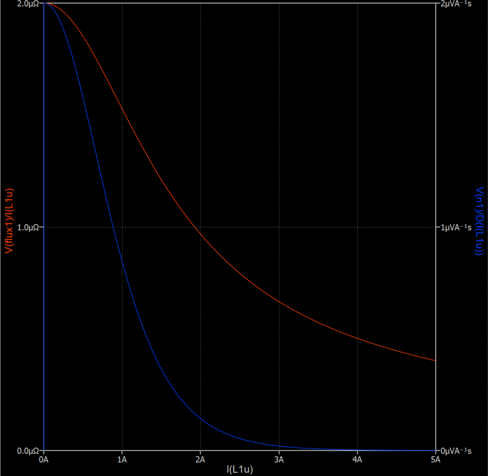
measure the voltage across the inductor when driven with a dI/dt = 1 A/s. The result in the plot is the BLUE waveform, being: V(n1)/D(I(L1u)). Even though in this case, having 1A/s, the division is redundant.
using a behavioural-voltage source which integrates the voltage across the inductor. Assuming N=1, this should be equal to the flux. Then, once I have the flux, I get the inductance value dividing by I(L).
The result is the RED waveform, being: V(flux)/I(L1u).

I see two problems here (but most likely I have mess something and it’s just under my nose):

First, is that the inductance values are equal at the peak, but they behave differently as you can see in the plot. The inductance value calculated as 2) is slow to converge to zero. Why is that? I thought that it may be due to some “integral effect”, but it’s only a gut feeling, I don’t find any justification for this. What is the most reliable estimation between the two?
Second problem I have is when I try to make the saturation steeper, by modifing the coefficients in the tanh() argument. For example, if I put Isat = 0.3 or equivalently tanh(3*x/Isat), the inductance is 3x the original value. I guess that what happens is that the derivative of flux is calculated, hence I have a 3x in the voltage across inductor. Is that correct?

In the end what I want to achieve is a reliable inductor model that can be used in a series magnetic compression simulation.
I also tried with flux={Lmax-Lsat}table(x, -{Isat},0, -{Isat0.9},1, 0,1, {Isat*0.9},1, {Isat},0), using a lookup table.
Well, in DC with monotone function (eg. increasing ramp) it works. But as soon as I drive it with an AC source, it gets stuck on discontinuity points. I was expecting that.

What can you suggest me?
thanks !

Ps. Since apparently I can’t upload the model, here’s the netlist:

ÿØÿÛ«schematic
«component (-1400,1200) 0 0
«symbol V
«type: V»
«description: Independent Voltage Source»
«shorted pins: false»
«line (0,-130) (0,-200) 0 0 0x1000000 -1 -1»
«line (0,200) (0,130) 0 0 0x1000000 -1 -1»
«rect (-25,77) (25,73) 0 0 0 0x1000000 0x3000000 -1 0 -1»
«rect (-2,50) (2,100) 0 0 0 0x1000000 0x3000000 -1 0 -1»
«rect (-25,-73) (25,-77) 0 0 0 0x1000000 0x3000000 -1 0 -1»
«ellipse (-130,130) (130,-130) 0 0 0 0x1000000 0x1000000 -1 -1»
«text (100,150) 1 7 0 0x1000000 -1 -1 “V1”»
«text (150,-150) 1 7 0 0x1000000 -1 -1 “sine 0 1 1K 0 0 0 2”»
«pin (0,200) (0,0) 1 0 0 0x0 -1 “+”»
«pin (0,-200) (0,0) 1 0 0 0x0 -1 “-”»
»
»
«component (1000,1200) 0 0
«symbol L
«type: L»
«description: Inductor»
«shorted pins: false»
«line (0,200) (0,180) 0 0 0x1000000 -1 -1»
«line (0,-200) (0,-180) 0 0 0x1000000 -1 -1»
«coil (-80,180) (80,-180) 0 0 0 0x1000000 -1 -1»
«text (150,150) 1 7 0 0x1000000 -1 -1 “L1u”»
«text (1345,-50) 1 15 0 0x1000000 -1 -1 “flux={Lmax}(tanh(10x/{Isat}))”»
«pin (0,200) (0,0) 1 0 0 0x0 -1 “1”»
«pin (0,-200) (0,0) 1 0 0 0x0 -1 “2”»
»
»
«component (-400,1600) 2 0
«symbol R
«type: R»
«description: Resistor(USA Style Symbol)»
«shorted pins: false»
«line (0,200) (0,180) 0 0 0x1000000 -1 -1»
«line (0,-180) (0,-200) 0 0 0x1000000 -1 -1»
«zigzag (-80,180) (80,-180) 0 0 0 0x1000000 -1 -1»
«text (80,0) 1 110 0 0x1000000 -1 -1 “R1”»
«text (-208,0) 1 111 0 0x1000000 -1 -1 “1”»
«pin (0,200) (0,0) 1 0 0 0x0 -1 “1”»
«pin (0,-200) (0,0) 1 0 0 0x0 -1 “2”»
»
»
«component (-1400,2900) 0 0
«symbol B1
«type: B»
«description: Behavioral Voltage Source»
«shorted pins: false»
«line (0,-130) (0,-200) 0 0 0x1000000 -1 -1»
«line (0,200) (0,130) 0 0 0x1000000 -1 -1»
«rect (-25,77) (25,73) 0 0 0 0x1000000 0x3000000 -1 0 -1»
«rect (-2,50) (2,100) 0 0 0 0x1000000 0x3000000 -1 0 -1»
«rect (-25,-73) (25,-77) 0 0 0 0x1000000 0x3000000 -1 0 -1»
«ellipse (-130,130) (130,-130) 0 0 0 0x1000000 0x1000000 -1 -1»
«text (100,150) 1 7 0 0x1000000 -1 -1 “B1”»
«text (100,-150) 1 7 0 0x1000000 -1 -1 “V=idt(V(N1),0)”»
«pin (0,200) (0,0) 1 0 0 0x0 -1 “+”»
«pin (0,-200) (0,0) 1 0 0 0x0 -1 “-”»
»
»
«component (-1400,600) 0 2
«symbol I
«type: I»
«description: Current Source»
«shorted pins: false»
«line (0,200) (0,150) 0 0 0x1000000 -1 -1»
«line (0,-150) (0,-200) 0 0 0x1000000 -1 -1»
«rect (-25,102) (25,98) 0 0 0 0x1000000 0x3000000 -1 0 -1»
«rect (-2,75) (2,125) 0 0 0 0x1000000 0x3000000 -1 0 -1»
«rect (-25,-98) (25,-102) 0 0 0 0x1000000 0x3000000 -1 0 -1»
«ellipse (-100,-150) (100,50) 0 0 0 0x1000000 0x1000000 -1 -1»
«ellipse (-100,-50) (100,150) 0 0 0 0x1000000 0x1000000 -1 -1»
«text (100,150) 1 7 0 0x1000000 -1 -1 “I1”»
«text (100,-150) 1 7 0 0x1000000 -1 -1 “PWL 0 -5 10 5”»
«pin (0,-200) (0,0) 1 0 0 0x0 -1 “-”»
«pin (0,200) (0,0) 1 0 0 0x0 -1 “+”»
»
»
«component (1000,300) 0 0
«symbol L
«type: L»
«description: Inductor»
«shorted pins: false»
«line (0,200) (0,180) 0 0 0x1000000 -1 -1»
«line (0,-200) (0,-180) 0 0 0x1000000 -1 -1»
«coil (-80,180) (80,-180) 0 0 0 0x1000000 -1 -1»
«text (100,150) 1 7 0 0x1000000 -1 -1 “L1”»
«text (100,-150) 1 7 0 0x1000000 -1 -1 “{Lsat}”»
«pin (0,200) (0,0) 1 0 0 0x0 -1 “1”»
«pin (0,-200) (0,0) 1 0 0 0x0 -1 “2”»
»
»
«net (-1400,-200) 1 13 0 “GND”»
«net (1000,1600) 1 14 0 “N1”»
«net (-1400,2600) 1 13 0 “GND”»
«net (-1400,3200) 1 14 0 “flux1”»
«junction (-1400,-100)»
«wire (-1400,800) (-1400,1000) “GND”»
«wire (1000,1400) (1000,1600) “N1”»
«wire (-600,1600) (-1400,1600) “N02”»
«wire (-1400,1600) (-1400,1400) “N02”»
«wire (-1400,-100) (1000,-100) “GND”»
«wire (-1400,-200) (-1400,-100) “GND”»
«wire (1000,1600) (-200,1600) “N1”»
«wire (-1400,2600) (-1400,2700) “GND”»
«wire (-1400,3200) (-1400,3100) “flux1”»
«wire (-1400,-100) (-1400,400) “GND”»
«wire (1000,100) (1000,-100) “GND”»
«wire (1000,1000) (1000,500) “N03”»
«text (-1600,5000) 1 7 0 0x1000000 -1 -1 “ï»¿.tran 1m”»
«text (-1600,4850) 1 7 0 0x1000000 -1 -1 “ï»¿.plot V(N1)/D(I(L1))”»
«text (350,4850) 1 7 0 0x1000000 -1 -1 “ï»¿;INDUTTANZA”»
«text (-1600,4700) 1 7 0 0x1000000 -1 -1 “ï»¿.param Isat=1 Lmax=2Âµ Lsat=200n”»
«text (-1450,2150) 1 7 0 0x1000000 -1 -1 “ï»¿;INDUTTANZA ARBITRARIA”»
«text (-1600,4150) 1 7 0 0x1000000 -1 -1 “ï»¿.options method=gear\n.options gmin=1e-9\n.options reltol=1e-3\n;.options maxstep=1n”»
«text (1200,2550) 1 7 0 0x1000000 -1 -1 “ï»¿;flux={Lmax-Lsat}table(x, -{Isat},0, -{Isat0.9},1, 0,1, {Isat*0.9},1, {Isat},0)”»
»

KSKelvin · March 25, 2025, 3:33pm

Not sure if this helps, but I included examples on nonlinear inductor with Isat, SATFRAC, Lsat, or Flux model in my GitHub “Device Reference Guide”, L. Inductor section.
https://github.com/KSKelvin-Github/Qspice/tree/main/Guideline

glon · March 27, 2025, 1:40pm

I’ll look into that. Thanks, KSKelvin.

mhx · March 28, 2025, 11:04am

Please note that these methods do not model the hysteresis of the core material, which for this application may be critical, as a lossless inductor with variable current dependent inductance violates conservation of energy laws. If it has to be LT/QSPICE based, maybe have a look at the Chan model (although it doesn’t model frequency dependent losses).